md

This keyword controls the details of the molecular dynamics (MD) simulation.

Options

type

Define the type of molecular dynamics (MD) simulation.

Value	`NVE`: Microcanonical ensemble; constant number of particles, volume, and energy.
	`NVT`: Canonical ensemble; constant number of particles, volume, and temperature.
	`fep-NVE`: Free energy perturbation calculation for the microcanonical ensemble.
	`fep-NVT`: Free energy perturbation calculation for the canonical ensemble.
Default	`NVE`

dt

The time step in picoseconds (ps). For systems that do not contain hydrogen atoms, dt can be set to 0.001 ps.

Value	A real number
Default	`0.0005`

num_steps

Specifies the number of MD steps to be run.
The total simulation time is dt × num_steps ps.

Value	An integer
Default	`10`

output_freq

The number of steps between outputs of MD information.
Trajectory, velocity, and gradient data will be written to disk.

Value	An integer
Default	`1`

temp

Defines the initial temperature for NVE simulations and the target temperature for NVT simulations.

Value	A real number
Default	`273.15`

temp_nhc_length

The length of the Nose–Hoover chain used to control the temperature. An integer greater than 2 is usually sufficient.

Value	An integer
Default	`5`

temp_nhc_tau

The time constant of the Nose–Hoover chain used to control the temperature, in picoseconds (ps).

Value	A real number
Default	`0.5`

vel_fn

If specified, the initial velocities will be read from the given XYZ file (in Å/ps). Otherwise, velocities will be generated from the Boltzmann distribution.

Value	A file name
Default	None

For example: initial velocities will be read from mol-vel.xyz.

md   
  vel_fn mol-vel.xyz
end

max_dr

The maximum allowed atomic displacement per step, in Ångström.
If any atom moves more than max_dr in a single step, Qbics will terminate the MD simulation, as such rapid motion may indicate an unstable or crashing system.

Value	A real number
Default	`5`

plumed_fn

Value	A file name
Default	None

If specified, Qbics will apply the enhanced sampling algorithms defined in this PLUMED input file.
For the input file syntax, please refer to the PLUMED manual.

Theoretical Background

Molecular Dynamics Simulations

Molecular dynamics (MD) simulations are a computational method used to study the time evolution of a system of interacting particles. In MD simulations, the forces between particles are calculated using a potential energy function, and the equations of motion are solved to obtain the particles' trajectories.
In Qbics, the equations of motion are solved using the velocity-Verlet algorithm, a symplectic integrator that conserves the total energy of the system over long timescales. Forces can be evaluated at various levels of theory, including DFT, MM, NDDO, xTB, DFT/MM, NDDO/MM, and xTB/MM.

During MD simulations, Qbics outputs four different files:

x-md-traj.xyz: The trajectory of the system in XYZ format.
x-md-vel.xyz: The velocities of the system in XYZ format.
x-md-grad.xyz: The gradients of the system in XYZ format. Note: force is the negative of the gradient.
x-md-log.txt: The log file of the MD simulation, containing step number, time, energy components, temperature, and other relevant information.

If plumed_fn is specified, Qbics will also output additional data as defined in the PLUMED input file.
Before running MD simulations, it is strongly recommended to perform a geometry optimization to obtain a stable initial configuration.

Each ensemble has its own conserved quantity.

For NVE, the total energy is conserved:

$$E = K + V$$

E is the total energy.
K is the kinetic energy.
V is the potential energy.

For example, if you run an NVE MD simulation, you can check the total energy in the file x-md-log.txt:

     #            Time                Total              Kinetic            Potential                 Temp  Cost
                    ps              Hartree              Hartree              Hartree               Kelvin  second
     0         0.00000         -34.44404963           0.02280104         -34.46685067         300.00000000  0.257
    20         0.01000         -34.44402464           0.01224859         -34.45627323         161.15837759  0.260
    40         0.02000         -34.44400898           0.01020550         -34.45421449         134.27682685  0.222
    60         0.03000         -34.44401439           0.01628312         -34.46029751         214.24190576  0.220
    80         0.04000         -34.44402295           0.02160569         -34.46562864         284.27246073  0.279
   100         0.05000         -34.44403491           0.03125266         -34.47528758         411.20057981  0.248
   120         0.06000         -34.44402767           0.02061378         -34.46464145         271.22164167  0.228
   140         0.07000         -34.44403668           0.02599444         -34.47003112         342.01656058  0.226
   160         0.08000         -34.44402275           0.01897475         -34.46299751         249.65643218  0.224

For NVT, the total “virtual” energy is conserved:

$$Q = K + V + \sum_{j=1}^{n_\text{NHC}} \frac{p_{\eta_j}^2}{2Q_j} + 3NkT\eta_1+kT \sum_{j=2}^{n_\text{NHC}}\eta_j$$

n_NHC is the Nose–Hoover chain length (nhc_temp_length).
k is the Boltzmann constant.
T is the temperature.
η_j and p_{η_j}are the thermostat variables ("position" and "momentum")
Q_jis the thermostat mass (automatically determined by Qbics).

For example, if you run an NVT MD simulation, you can check the ConstQ value in the file x-md-log.txt:

     #            Time                Total              Kinetic            Potential                 Temp               ConstQ  Cost
                    ps              Hartree              Hartree              Hartree               Kelvin              Hartree  second
     0         0.00000         -34.44404963           0.02280104         -34.46685067         300.00000000         -34.44404963  0.000
    20         0.01000         -34.44404123           0.01734433         -34.46138557         228.20455596         -34.44404256  0.293
    40         0.02000         -34.44401539           0.01535660         -34.45937199         202.05137626         -34.44402161  0.230
    60         0.03000         -34.44399789           0.01914301         -34.46314090         251.87027197         -34.44401529  0.213
    80         0.04000         -34.44401533           0.03373382         -34.47774915         443.84591789         -34.44404524  0.303
   100         0.05000         -34.44399074           0.01808475         -34.46207549         237.94640025         -34.44402711  0.222
   120         0.06000         -34.44400165           0.03088255         -34.47488420         406.33083745         -34.44404511  0.218
   140         0.07000         -34.44397432           0.01350937         -34.45748370         177.74683071         -34.44402030  0.327
   160         0.08000         -34.44397272           0.01886731         -34.46284002         248.24278233         -34.44402353  0.222
   180         0.09000         -34.44398418           0.03438731         -34.47837149         452.44411562         -34.44404296  0.225

In all cases, if the conserved quantity is not maintained, it indicates that the simulation is unstable. You may need to:

Reduce the time step;
Perform a geometry optimization to obtain a stable initial configuration;
Check whether the potential energy function (quantum chemistry or force field parameters) is appropriate for your system.

However, if plumed_fn is specified, the conserved quantity may not be preserved, as the enhanced sampling algorithm can alter the total energy.

Nose-Hoover Chain algorithm

The Nose–Hoover chain (NHC) algorithm is a method used to control the temperature in MD simulations. It is a generalization of the Nose–Hoover thermostat, consisting of a series of thermostats connected in sequence. The first thermostat controls the temperature of the system, while each subsequent thermostat controls the temperature of the preceding one.
The length of the NHC is controlled by temp_nhc_length, which should be greater than 2.
If temp_nhc_length is set to 1, the system may not produce a correct canonical distribution of velocities.

Input Examples

Example: Dynamic Effects in a Carbocation Reaction

Consider the following reaction:
We want to determine which group is more likely to migrate. To investigate this, we will perform a 200 fs NVT MD simulation starting from the optimized structure of the carbocation. The simulation will be repeated 20 times using a shell script run.sh. Here, we use xTB due to its computational efficiency, though DFT can also be used if sufficient time and resources are available.
The input files are shown below:

mol
    C    -0.90849     0.15356    -0.48118
    C    -0.18840    -0.79035     0.24223
    C    -0.79661    -1.92884     0.73482
    C    -2.15434    -2.10431     0.51590
    C    -2.88201    -1.15101    -0.17642
    C    -2.26735    -0.01407    -0.67971
    H    -0.22972    -2.66722     1.27887
    H    -2.64692    -2.98493     0.89733
    H    -3.93966    -1.29437    -0.33076
    H    -2.84788     0.72259    -1.21038
    C     1.26411    -0.39651     0.38023
    C    -0.02903     1.30229    -0.93562
    C     1.67317    -0.22550     1.85240
    H     1.83624    -1.21169     2.27913
    H     2.60525     0.32605     1.95669
    H     0.88426     0.23363     2.45602
    C    -0.71228     2.64784    -0.65267
    H    -0.02047     3.48874    -0.70508
    H    -1.46470     2.82054    -1.41711
    H    -1.26222     2.63862     0.29289
    C     1.31204     0.95650    -0.38570
    H     2.18545     1.61818    -0.54700
    C     2.13967    -1.43173    -0.30477
    H     1.61435    -2.09539    -0.97595
    C     3.43556    -1.57292    -0.10516
    H     3.99105    -2.34108    -0.61298
    H     4.00084    -0.94936     0.56664
    C     0.38001     1.16971    -2.43593
    C     1.13470     2.39986    -2.94354
    C    -0.80675     0.90408    -3.35872
    H     1.04783     0.30446    -2.50076
    H     1.96481     2.68234    -2.30028
    H     1.54266     2.18219    -3.92659
    H     0.47031     3.25225    -3.05019
    H    -1.34333     0.00481    -3.07250
    H    -1.49736     1.74331    -3.36799
    H    -0.44263     0.76667    -4.37283
end

basis
    def2-svp
end

pseudopotential
    def2-ecp
end

scf
    charge  +1
    spin2p1  1
end

xtb
    chrg +1
end

md
    type            nvt
    dt              0.001  # 0.001 ps = 1 fs
    num_steps       200    # 0.001*200 = 0.2 ps. In real simultion, you may need > 1 ps.
    temp            300
    temp_nhc_length 5
    temp_nhc_tau    0.5
    output_freq     10     # 0.001*10 = 10 fs
end

task
    md xtb
    # md m06 # If you want to use DFT.
end

for i in {1..20}; do
    fn=md-1-$i
    cp md-1.inp ${fn}.inp
    qbics ${fn}.inp -n 8 > ${fn}.out
done

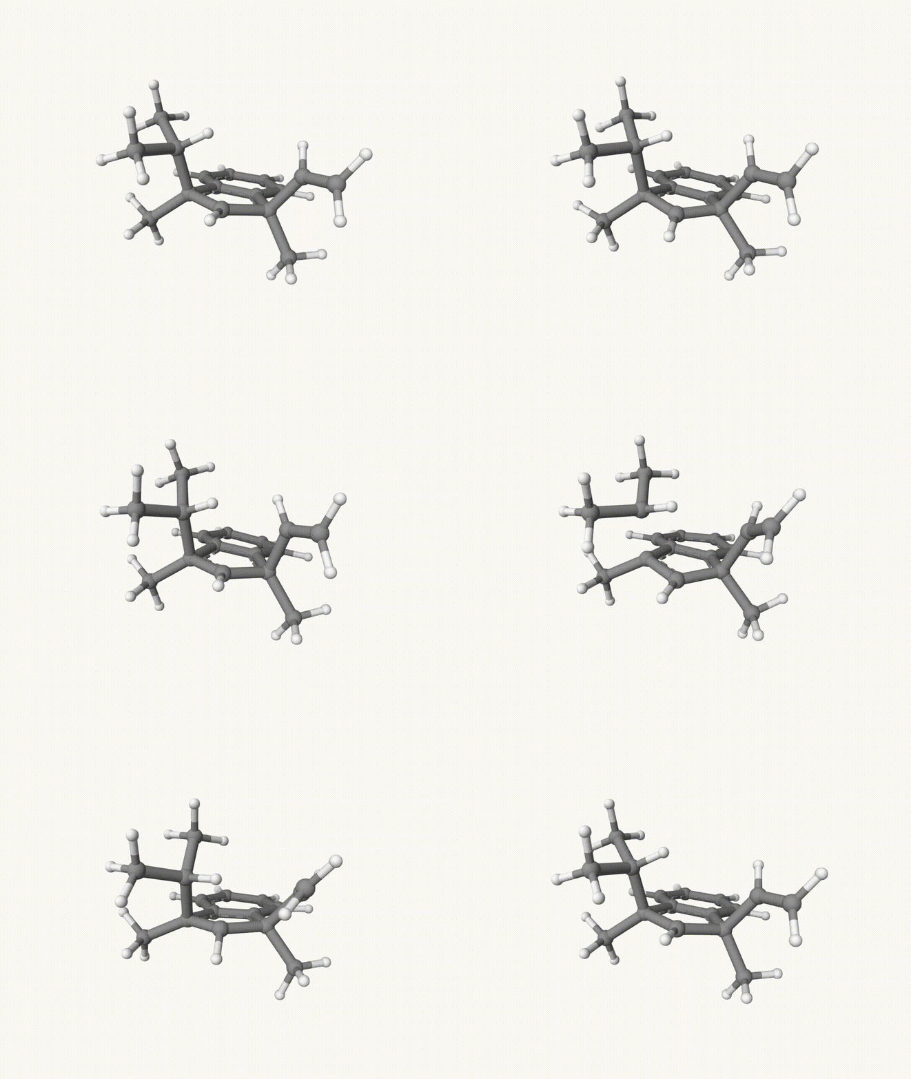
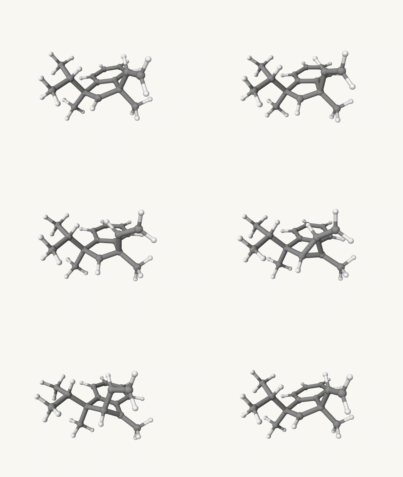
By bash run.sh, you can run 20 MD simulations. The output files will be md-1-1-md-traj.xyz, etc. We observe that both the isopropyl and vinyl group can migrate. For example:

For this test, we calculate the migration ratio of the isopropyl group to the vinyl group.
Based on 20 trajectories, the result is:

Isopropyl group migration	7
Vinyl group migration	7
Non-reactive	2
Other reactions	4

Of course, if the simulation time is extended, a non-reactive trajectory may become reactive.
Nevertheless, the NVT MD results suggest that the migration ratio is approximately 1:1.
Why do we perform dynamics? Due to the nonstatistical nature of this reaction, the migration ratio cannot be accurately predicted by static calculations.
The results from dynamics are more reliable. For more details, please refer to: J. Am. Chem. Soc. 2021, 143, 1088

md