Tip
All input files can be downloaded: Files.
Tip
For more information of this section, please refer to these pages:
MSDFT (2): Core Ionizations and Excitations
This tutorial will lead you step by step to study excited states using Multi-State Density Functional Theory (MSDFT).
MSDFT is a powerful method for studying excited states. It optimizes excited states using TSO-DFT method, so it is free of orbital relaxation problem like in TDDFT. In this section, you will see that MSDFT can give much more reasonable results than TDDFT for excited states.
In TSO-DFT (1): Excited States, we have introduced how to use TSO-DFT to study excited states. In MSDFT (1): All Types of Excited States, we have introduced how to use MSDFT to study excitations generally. In this tutorial, we will introduce how to use MSDFT to study core excitations. We strongly recommend you to read these two tutorials before reading this tutorial.
Actually, MSDFT can be considered as TSO+NOSI. MSDFT is a framework that automaitcally performs TSO-DFT and NOSI for required excited states. Of course, you can also perform TSO-DFT and NOSI separately for special purposes.
Example: Core Ionization Poteitals of CH3CN
Tip
To study core excitations, one should use the (aug-)cc-pCVXZ basis set here instead of the (aug-)cc-pVXZ basis set for heavy atoms.
Before going to core excitations, we first discuss how to calculate the core ionization potentials.
First, we do a ground state calculation for CH3CN.
 1basis
 2    element
 3    H cc-pVTZ
 4    N cc-pCVTZ
 5    C cc-pCVTZ
 6end
 7
 8scf
 9    charge  0
10    spin2p1 1
11    type    u
12end
13
14mol
15    C     -0.04745178     -0.06805384     -0.11694780
16    H      0.30905509     -1.09741742     -0.13005981
17    H      0.30945822      0.43682112     -1.01404303
18    H     -1.13674654     -0.07474849     -0.12959758
19    C      0.43731777      0.61649095      1.07195392
20    N      0.81994723      1.16084767      2.00936430
21end
22
23task
24    energy b3lyp
25end
Note that, to study core excitations, we need to use a basis set that can describe core orbitals well. So we use the cc-pCVTZ basis set here instead of the cc-pVTZ basis set for heavy atoms. For hydrogen atoms, we use the cc-pVTZ basis set.
In the outpuf wave function file msdft-2-gs.mwfn, we can see the core orbitals are the 1s orbitals of carbon and oxygen atoms using Qbics-MolStar. First drag msdft-2-gs.mwfn into explorer, and it will be automatically loaded. Right-click msdft-2-gs.mwfn and select View Molecular Orbitals, click orbital 1, 2, and 3:
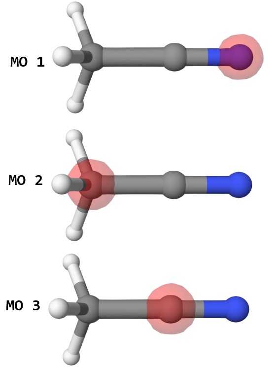
Thus, the MO 1,2,3 are the 1s orbitals of nitrogen, methyl group carbon, and cyano group carbon atom, respectively. We will calculate the core ionization potentials of these 3 orbitals. The input file are:
 1basis
 2    element
 3    H cc-pVTZ
 4    N cc-pCVTZ
 5    C cc-pCVTZ
 6end
 7
 8scf
 9    charge  0
10    spin2p1 1
11    type    u
12    no_scf  tso
13end
14
15scfguess
16    type mwfn
17    file msdft-2-gs.mwfn
18    orb 21 2     1-170 : 2-171
19    orb 0  1       171 : 1
20end
21
22mol
23    C     -0.04745178     -0.06805384     -0.11694780
24    H      0.30905509     -1.09741742     -0.13005981
25    H      0.30945822      0.43682112     -1.01404303
26    H     -1.13674654     -0.07474849     -0.12959758
27    C      0.43731777      0.61649095      1.07195392
28    N      0.81994723      1.16084767      2.00936430
29end
30
31task
32    energy b3lyp
33end
 1basis
 2    element
 3    H cc-pVTZ
 4    N cc-pCVTZ
 5    C cc-pCVTZ
 6end
 7
 8scf
 9    charge  0
10    spin2p1 1
11    type    u
12    no_scf  tso
13end
14
15scfguess
16    type mwfn
17    file msdft-2-gs.mwfn
18    orb 21 2   1-170 : 1 3-171
19    orb 0  1     171 : 2
20end
21
22mol
23    C     -0.04745178     -0.06805384     -0.11694780
24    H      0.30905509     -1.09741742     -0.13005981
25    H      0.30945822      0.43682112     -1.01404303
26    H     -1.13674654     -0.07474849     -0.12959758
27    C      0.43731777      0.61649095      1.07195392
28    N      0.81994723      1.16084767      2.00936430
29end
30
31task
32    energy b3lyp
33end
 1basis
 2    element
 3    H cc-pVTZ
 4    N cc-pCVTZ
 5    C cc-pCVTZ
 6end
 7
 8scf
 9    charge  0
10    spin2p1 1
11    type    u
12    no_scf  tso
13end
14
15scfguess
16    type mwfn
17    file msdft-2-gs.mwfn
18    orb 21 2   1-170 : 1 2 4-171
19    orb 0  1     171 : 3
20end
21
22mol
23    C     -0.04745178     -0.06805384     -0.11694780
24    H      0.30905509     -1.09741742     -0.13005981
25    H      0.30945822      0.43682112     -1.01404303
26    H     -1.13674654     -0.07474849     -0.12959758
27    C      0.43731777      0.61649095      1.07195392
28    N      0.81994723      1.16084767      2.00936430
29end
30
31task
32    energy b3lyp
33end
Let us take msdft-2-ip1.inp as an example. As all basis set and coordinates are the same as the ground state calculation, we only need to change the orbital to be calculated. We use TSO-DFT to calculate the core ionization potential of the 1s orbital of nitrogen atom.
Line 16,17: we will use the ground state wave function file
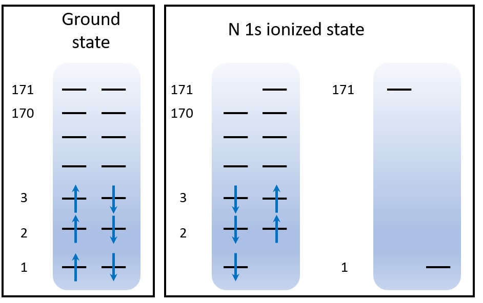
msdft-2-gs.mwfnto generate the initial guess for the ionized state calculation.Line 18: we build a orbital space containing alpha orbitals 1-171, and beta orbitals 2-170. Note that, the number of electrons is only
21instead of22in neutral state, so the spin multiplicity is2instead of1. Note that, with this orbital space, elecrons are automatically assigned to the corresponding orbitals with the nitrogen 1s alpha orbital unoccupied.Line 19: a remaining orbital space containing only the nitrogen 1s beta orbital is specified and the highest alpha orbital to keep the numbers of alpha and beta orbitals the same.
The orbital space is shown below. You can also see TSO-DFT (1): Excited States for more details about the orbital space.
After calculation, the output is shown below:
1TSO Transition
2==============
3Reference wave function read from: msdft-2-gs.mwfn
4Reference energy:         -132.81032200 Hartree
5Current energy:           -117.91513595 Hartree
6E(Current)-E(Ref):         405.31865749 eV
1TSO Transition
2==============
3Reference wave function read from: msdft-2-gs.mwfn
4Reference energy:         -132.81032200 Hartree
5Current energy:           -122.05195311 Hartree
6E(Current)-E(Ref):         292.75012878 eV
1TSO Transition
2==============
3Reference wave function read from: msdft-2-gs.mwfn
4Reference energy:         -132.81032200 Hartree
5Current energy:           -122.05109782 Hartree
6E(Current)-E(Ref):         292.77340232 eV
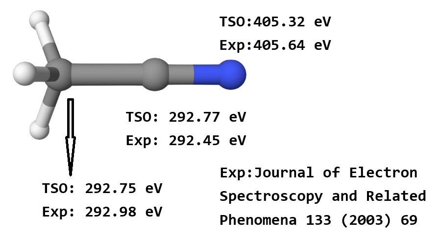
The hightlighted values are the core ionization potentials of the 1s orbitals of nitrogen, methyl group carbon, and cyano group carbon atom, respectively. The results from TSO-DFT are very accurate, see below:
Example: C and N K-edge XAS of CH3CN
Now we can calculate 1s excitation energies, i.e. K-edge XAS. The energy range of C (292 eV) and N (402 eV) K-edge XAS are quiet separated, so we can use 2 files to calculate them. See below:
 1basis
 2    element
 3    H cc-pVTZ
 4    N cc-pCVTZ
 5    C cc-pCVTZ
 6end
 7
 8scf
 9    charge  0
10    spin2p1 1
11    type    u
12    schwarz 1.E-14
13end
14
15output
16    not_strict
17end
18
19mol
20    C     -0.04745178     -0.06805384     -0.11694780
21    H      0.30905509     -1.09741742     -0.13005981
22    H      0.30945822      0.43682112     -1.01404303
23    H     -1.13674654     -0.07474849     -0.12959758
24    C      0.43731777      0.61649095      1.07195392
25    N      0.81994723      1.16084767      2.00936430
26end
27
28msdft
29    single_ex 2-3 : 12-16
30end
31
32task
33    msdft b3lyp
34end
 1basis
 2    element
 3    H cc-pVTZ
 4    N cc-pCVTZ
 5    C cc-pCVTZ
 6end
 7
 8scf
 9    charge  0
10    spin2p1 1
11    type    u
12    schwarz 1.E-14
13end
14
15output
16    not_strict
17end
18
19mol
20    C     -0.04745178     -0.06805384     -0.11694780
21    H      0.30905509     -1.09741742     -0.13005981
22    H      0.30945822      0.43682112     -1.01404303
23    H     -1.13674654     -0.07474849     -0.12959758
24    C      0.43731777      0.61649095      1.07195392
25    N      0.81994723      1.16084767      2.00936430
26end
27
28msdft
29    single_ex 1 : 12-16
30end
31
32task
33    msdft b3lyp
34end
Take msdft-2-CXAS.inp as an example. The MSDFT option:
msdft...endindicates the MSDFT calculation. Here,single_ex 2-3 : 12-16means we want to study the single excitation from orbitals 2,3 to orbitals 12 to 16. Explicitly, we want to study the following single excitations:2 → 12
2 → 13
2 → 14
2 → 15
2 → 16
3 → 12
3 → 13
3 → 14
3 → 15
3 → 16
msdft-2-NXAS.inp is similar.
After calculation, the output is shown below:
 1---- NOSI Results ----
 2======================
 3   State   NOSI Energies  Excited Energy       Osc. Str.        DX        DY        DZ
 4               (Hartree)            (eV)                    (a.u.)    (a.u.)    (a.u.)
 5       0   -132.81033068      0.00000000      0.00000000  20.96814  29.62520  51.36982
 6       1   -122.29776407    286.04693739      0.00000000  -0.00000   0.00000  -0.00000
 7       2   -122.29628111    286.08728868      0.00000000   0.00000  -0.00000   0.00000
 8       3   -122.27262763    286.73090010      0.06090910   0.00031  -0.11416   0.06602
 9       4   -122.27184218    286.75227222      0.06054746  -0.12395   0.02131   0.03833
10       5   -122.22807524    287.94317052      0.00000000  -0.00000  -0.00000  -0.00000
11       6   -122.20022633    288.70093945      0.00148936  -0.00675   0.00366   0.01906
12       7   -122.19999870    288.70713325      0.00000000   0.00000  -0.00000   0.00000
13       8   -122.19931169    288.72582670      0.00000000   0.00000  -0.00000  -0.00000
14       9   -122.19077081    288.95822418      0.01841754  -0.00426   0.06444  -0.03238
15      10   -122.18956504    288.99103317      0.01846930  -0.06940   0.00640   0.01937
16      11   -122.13308009    290.52798857      0.00000000   0.00000   0.00000  -0.00000
17      12   -122.12598852    290.72095017      0.00000000  -0.00000  -0.00000   0.00000
18      13   -122.12277134    290.80848975      0.02666731   0.07435  -0.04434  -0.00365
19      14   -122.11545370    291.00760270      0.02780428   0.03543   0.06347  -0.05038
20      15   -122.08534743    291.82679427      0.00000000   0.00000  -0.00000   0.00000
21      16   -122.08400221    291.86339771      0.00255869   0.02421  -0.01085  -0.00373
22      17   -122.08280065    291.89609221      0.00000000   0.00000  -0.00000   0.00000
23      18   -122.08151697    291.93102093      0.00252312   0.00672   0.02049  -0.01558
24      19   -121.85348605    298.13574240      0.00040867   0.00666  -0.00638  -0.00521
25      20   -121.84404145    298.39272982      0.00000000   0.00000   0.00000  -0.00000
26
27---- NOSI State Identification (Coefficients) ----
28==================================================
29State |0> = +1.000 |msdft-2-CXAS-gs.mwfn>
30State |1> = -0.487 |msdft-2-CXAS-3-to-12-se.mwfn> +0.487 |spin_flip_msdft-2-CXAS-3-to-12-se.mwfn> +0.419 |          msdft-2-CXAS-3-to-13-se.mwfn> -0.419 |spin_flip_msdft-2-CXAS-3-to-13-se.mwfn>
31State |2> = +0.314 |msdft-2-CXAS-3-to-12-se.mwfn> -0.314 |spin_flip_msdft-2-CXAS-3-to-12-se.mwfn> +0.461 |          msdft-2-CXAS-3-to-13-se.mwfn> -0.461 |spin_flip_msdft-2-CXAS-3-to-13-se.mwfn> +0.311 |msdft-2-CXAS-3-to-14-se.mwfn>           -0.311 |spin_flip_msdft-2-CXAS-3-to-14-se.mwfn>
32State |3> = -0.445 |msdft-2-CXAS-3-to-12-se.mwfn> -0.445 |spin_flip_msdft-2-CXAS-3-to-12-se.mwfn> +0.372 |          msdft-2-CXAS-3-to-13-se.mwfn> +0.372 |spin_flip_msdft-2-CXAS-3-to-13-se.mwfn> -0.041 |msdft-2-CXAS-3-to-14-se.mwfn>           -0.041 |spin_flip_msdft-2-CXAS-3-to-14-se.mwfn>
33State |4> = +0.086 |msdft-2-CXAS-3-to-12-se.mwfn> +0.086 |spin_flip_msdft-2-CXAS-3-to-12-se.mwfn> +0.479 |          msdft-2-CXAS-3-to-13-se.mwfn> +0.479 |spin_flip_msdft-2-CXAS-3-to-13-se.mwfn> +0.458 |msdft-2-CXAS-3-to-14-se.mwfn>           +0.458 |spin_flip_msdft-2-CXAS-3-to-14-se.mwfn>
34State |5> = +0.706 |msdft-2-CXAS-2-to-12-se.mwfn> -0.706 |spin_flip_msdft-2-CXAS-2-to-12-se.mwfn>
35State |6> = -0.696 |msdft-2-CXAS-2-to-12-se.mwfn> -0.696 |spin_flip_msdft-2-CXAS-2-to-12-se.mwfn>
 1---- NOSI Results ----
 2======================
 3   State   NOSI Energies  Excited Energy       Osc. Str.        DX        DY        DZ
 4               (Hartree)            (eV)                    (a.u.)    (a.u.)    (a.u.)
 5       0   -132.81032203      0.00000000      0.00000000  20.96814  29.62523  51.36982
 6       1   -118.14811920    398.95853898      0.00000000  -0.00000   0.00000  -0.00000
 7       2   -118.14680628    398.99426361      0.00000000   0.00000  -0.00000   0.00000
 8       3   -118.12556491    399.57224120      0.05264859   0.08930  -0.05270  -0.00609
 9       4   -118.12410116    399.61206995      0.05267515   0.04016   0.07493  -0.05970
10       5   -117.94199382    404.56721069      0.00000000   0.00000  -0.00000  -0.00000
11       6   -117.94127276    404.58683066      0.00171928  -0.01720   0.00646   0.00323
12       7   -117.93957743    404.63296056      0.00000000  -0.00000  -0.00000   0.00000
13       8   -117.93889138    404.65162785      0.00169993  -0.00377  -0.01499   0.01025
14       9   -117.81947316    407.90099772      0.00011256   0.00131  -0.00341  -0.00304
15      10   -117.81277843    408.08316134      0.00000000   0.00000   0.00000  -0.00000
16
17---- NOSI State Identification (Coefficients) ----
18==================================================
19State |0> = +1.000 |msdft-2-NXAS-gs.mwfn>
20State |1> = -0.530 |msdft-2-NXAS-1-to-12-se.mwfn> +0.530 |spin_flip_msdft-2-NXAS-1-to-12-se.mwfn> +0.360 |msdft-2-NXAS-1-to-13-se.mwfn> -0.360 |spin_flip_msdft-2-NXAS-1-to-13-se.mwfn>
21State |2> = +0.542 |msdft-2-NXAS-1-to-12-se.mwfn> -0.542 |spin_flip_msdft-2-NXAS-1-to-12-se.mwfn> +0.617 |msdft-2-NXAS-1-to-13-se.mwfn> -0.617 |spin_flip_msdft-2-NXAS-1-to-13-se.mwfn>
22State |3> = +0.390 |msdft-2-NXAS-1-to-12-se.mwfn> +0.390 |spin_flip_msdft-2-NXAS-1-to-12-se.mwfn> -0.336 |msdft-2-NXAS-1-to-13-se.mwfn> -0.336 |spin_flip_msdft-2-NXAS-1-to-13-se.mwfn> -0.133 |msdft-2-NXAS-1-to-14-se.mwfn> -0.133 |spin_flip_msdft-2-NXAS-1-to-14-se.mwfn>
23State |4> = -0.526 |msdft-2-NXAS-1-to-12-se.mwfn> -0.526 |spin_flip_msdft-2-NXAS-1-to-12-se.mwfn> -0.621 |msdft-2-NXAS-1-to-13-se.mwfn> -0.621 |spin_flip_msdft-2-NXAS-1-to-13-se.mwfn>
The excitation energies, oscillator strengths, and transition dipole moments, and state coefficients can be found here and details can be found in MSDFT (1): All Types of Excited States.
You can use the python script provided in qbics/tools/plotspec.py to plot the XAS spectra for msdft-2-CXAS-spectrum.txt and msdft-2-NXAS-spectrum.txt. Copy it to the same directory as the output files, and modify the parameters according to the introductions in MSDFT (1): All Types of Excited States. For example, to plot the C K-edge XAS spectrum, use:
1if __name__ == "__main__":
2    fn = "msdft-2-CXAS-spectrum.txt" # Spectrum file name.
3    eL_eV = 286                 # Lower energy limit.
4    eH_eV = 298                 # Higher energy limit.
5    sigma_eV = 0.2              # Sigma value.
6    num_ps = 3000                # Number of points.
7    use_angle = False           # Whether to use angle dependence.
1if __name__ == "__main__":
2    fn = "msdft-2NXAS-spectrum.txt" # Spectrum file name.
3    eL_eV = 308                 # Lower energy limit.
4    eH_eV = 408                 # Higher energy limit.
5    sigma_eV = 0.2              # Sigma value.
6    num_ps = 3000                # Number of points.
7    use_angle = False           # Whether to use angle dependence.
The spectra are shown below:
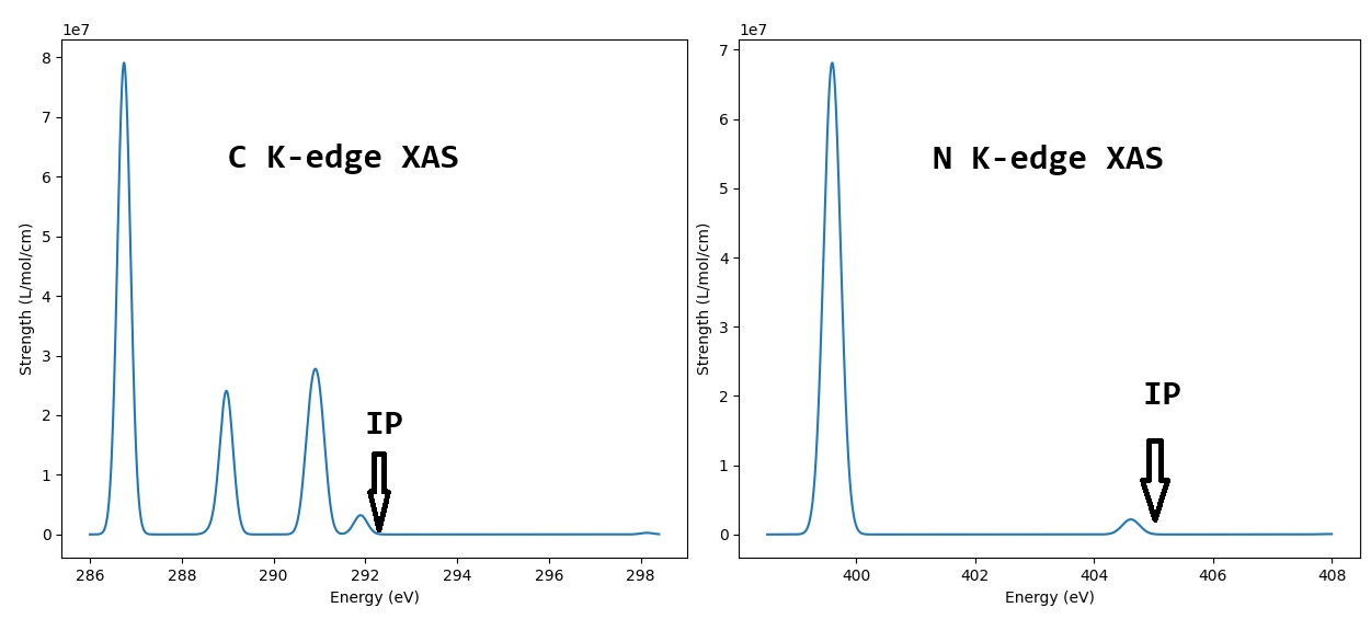
Tip
Note that in XAS we indicate the position of IP. This also reminds you that it is NOT necessary to calculate core excitated states beyond this IP. Beyond this IP, an accurate calculation of the excitation involves the use of continuous states, which is not considered in this tutorial.
You can try to identify the spectrum. For example, the largest peak in N K-edge XAS is 399.5 eV, which corresponds state 3 and 4 in msdft-2-NXAS.out (see highlighted lines), and the peak turns out to be a mixture of N(1s) → 12(LUMO) and N(1s) → 13(LUMO+1) transitions.