Tip

All input files can be downloaded: Files.

Tip

For more information of this section, please refer to these keywords:

• md

• Plumed documentation

Metadynamics for Calculating Free Energy Surface

This tutorial will lead you step by step to do molecular dynamics (MD) simulations with enhanced sampling using Qbics. We recommend you read Standard Molecular Dynamics Simulations first.

Enhanced samping is a method to sample rare events in MD simulations, mostly the overcome of high barrier, including difficult conformational change and chemical reactions. This is not a black-box method and you need some experience to select collective variables (CVs) and sampling methods. In Qbics, enhanced sampling is implemented with Plumed. All CVs and sampling methods in Plumed can be used. They can be combined with (TSO-)DFT, xTB, NDDO, CHARMM, and QM/MM in Qbics. In this tutorial, we will focus on metadynamics, although other methods like OPES can also be used.

Example: Conformation Change of Dialaline

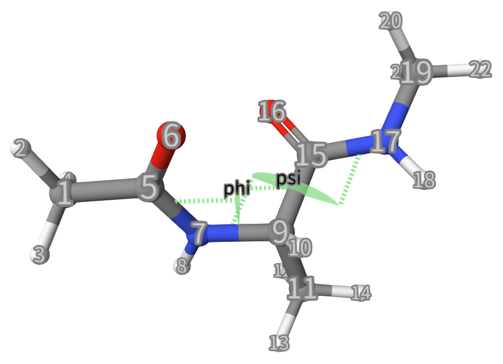
Here, we want to calculate the free energy surface (FES) of 2 dihedral angles (phi and psi) for dialaline with CHARMM force field, see below:

We will use metadynamics, which will add a bias potential to the place it has visited:

\[V(\mathbf{s},t) = \sum_{ k \tau < t} W(k \tau) \exp\left( -\sum_{i=1}^{d} \frac{(\mathbf{s}_i-\mathbf{s}_i^{(0)}(k \tau))^2}{2\sigma_i^2} \right)\]

Here, \(\mathbf{s}\) is the collective variables, \(t\) is the time, \(\tau\) is the time step, \(W(k \tau)\) is the height of the bias potential, \(\sigma_i\) is the width of the bias potential, \(k\) is the frequency of adding bias potential.

The input file for Qbics is almost same as standard MD simulations:

diala.inp

charmm
    parameters par_all22_prot.prm   # Parameter files. There can be several ones.
    topology   diala.psf            # Topology file.
    scaling14  1.0                  # Scaling factor of 1-4 interactions.
    rcutoff    12.0                 # The cutoff radius for nonbonded interactions.
    rswitch    10.0
end

mol
    diala.pdb
end

md
    type              NVT      # Type: NVE, NVT
    dt                0.001    # The time step in ps.
    temp              300.     # The temperature in Kelvin.
    temp_nhc_length   5        # The length of temperature Nose-Hoover chain.
    temp_nhc_tau      0.2      # The time constant of temperature Nose-Hoover chain in ps.
    num_steps         10000000 # The number of steps: 10 ns
    output_freq       100000   # The output frequency: 0.1 ns
    plumed_fn         plumed.dat # Plumed settings file.
end

task
    md charmm
end

The only difference is the addition of plumed_fn in md...end, which is the file that contains the settings for Plumed. With plumed_fn added, enhanced sampling will be automatically activated; if you delete this line, an ordinary MD simulation will be performed.

We can see that a 100 ns NVT MD will be carried out with enhanced sampling set in plumed.dat:

plumed.dat

# Compute the backbone dihedral angle phi, defined by atoms C-N-CA-C
phi: TORSION ATOMS=5,7,9,15
psi: TORSION ATOMS=7,9,15,17

metad: METAD ...
   ARG=phi,psi
   SIGMA=0.20,0.20
   HEIGHT=0.0836799999612436
   #BIASFACTOR=5
   #TEMP=300.0
   PACE=100
   FILE=HILLS
   GRID_MIN=-pi,-pi
   GRID_MAX=pi,pi
   #GRID_BIN=150,150
...

# Print both collective variables on COLVAR file every 10 steps
PRINT ARG=phi,psi FILE=COLVAR STRIDE=10

More details about Plumed can refer to Plumed documentation. Here, we give some explainations:

• Line 1: A comment.

• Line 2: Defines a CV named phi. The TORSION keyword specifies that this CV is a dihedral angle (the angle between two planes formed by four atoms). ATOMS=5,7,9,15 lists the indices (5, 7, 9, 15) of the four atoms in the simulation system that form the phi dihedral angle. See the figure below.

• Line 3: Similar to Line 2.

• Line 5: metad: METAD ... Starts the definition of a metadynamics simulation block named metad (the METAD keyword initializes metadynamics). The ... is a line continuation marker, indicating the configuration for this metadynamics block continues on the next lines.

• Line 6: Specifies the CVs to be used in metadynamics. Here, ARG=phi,psi means the metadynamics simulation will bias the system based on the two dihedral angles phi and psi. This is \(\mathbf{s} = (\phi, \psi)\) in the equation above.

• Line 7: Sets the width (Gaussian width) of the bias potentials added in metadynamics. The two values 0.20,0.20 correspond to the \(\sigma_i\) for phi and psi respectively (units are typically radians for angles), controlling how “spread out” each added Gaussian bias is.

• Line 8: Defines the height of each Gaussian bias potential added during metadynamics. The value 0.0836799999612436 (units are typically in energy units like kilojoules per mole, kJ/mol) determines how strong each individual bias contribution is. This is \(W(k \tau)\) in the equation above.

• Line 9: Set the BIASFACTOR (a parameter sometimes used to scale the bias potential) to 5. It is currently commented out.

• Line 10: Specify the simulation temperature (TEMP) as 300.0 Kelvin (K) for metadynamics calculations if uncommented. It is currently commented out.

• Line 11: Sets the frequency at which Gaussian bias potentials are added, which is \(k\) in the equation above. PACE=100 means a new Gaussian bias is added every 100 MD steps. In our case, 100*0.001 = 0.1 ps.

• Line 12: Specifies the output file where information about the added Gaussian biases (called “hills” in metadynamics) is stored. The file named HILLS will record details like the position, height, and width of each added hill for later analysis.

• Line 13: Defines the minimum bounds of the grid used for analyzing or visualizing the metadynamics FES. The values -pi,-pi (in radians) set the lower limit for the phi and psi CVs respectively (equivalent to -180 degrees).

• Line 14: Similar to Line 13, but defines the maximum bounds of the FES grid.

• Line 15: Set the number of grid bins (resolution) for the FES. GRID_BIN=150,150 would divide the phi and psi ranges into 150 bins each (resulting in a 150x150 grid). It is currently commented out.

• Line 16: Ends the line continuation for the metad metadynamics block, closing the configuration for this section.

• Line 19: Defines an output section using the PRINT keyword. ARG=phi,psi specifies the CVs to print (phi and psi), FILE=COLVAR sets the output file name to COLVAR, and STRIDE=10 means the CV values are written to COLVAR every 10 MD steps.

Attention

In Plumed, the default units for length, degree, and energy is nm, radian, and kJ/mol, not Angstrom, degree, and kcal/mol used in Qbics.

With this input files, we can run a 100-ns metadynamics simulation for dialaline.

After the simulation, a file named HILLS will be generated. It saves all \(V(\mathbf{s},t)\) during simulation, with which we can generate free energy data (FES) using the following command:

plumed sum_hills --hills HILLS

The executable of Plumed can be found in plumed/bin in the distribution of Qbics. This will generate the file fes.dat. With the following Python script, we can plot the FES \(F(\phi, \psi)\):

plot_fes.py

import numpy as np
import matplotlib.pyplot as plt
from matplotlib import cm

def plot_contour_from_file(filename):
    # Read file.
    data = np.loadtxt(filename)
    x = data[:, 0]
    y = data[:, 1]
    z = data[:, 2]
    x_unique = np.unique(x)
    y_unique = np.unique(y)
    # Create grids.
    X, Y = np.meshgrid(x_unique, y_unique)
    Z = np.zeros_like(X)
    for i, xi in enumerate(x_unique):
        for j, yi in enumerate(y_unique):
            mask = (x == xi) & (y == yi)
            if np.any(mask):
                Z[j, i] = z[mask][0]
    X *= 180/3.1415926 # To degree
    Y *= 180/3.1415926 # To degree
    Z *= 0.23900574    # To kcal/mol
    # Plot.
    plt.figure(figsize=(10, 8))
    contourf = plt.contourf(X, Y, Z, levels=25, cmap='jet')
    contour = plt.contour(X, Y, Z, levels=25, colors='black', linewidths=1)
    # Style.
    cbar = plt.colorbar(contourf)
    cbar.set_label('$F(\phi, \psi)$ (kcal/mol)', fontsize=12)
    plt.xlabel('$\phi$ (degree)', fontsize=12)
    plt.ylabel('$\psi$ (degree)', fontsize=12)
    plt.title('Free Energy Surface $F(\phi, \psi)$', fontsize=14)
    plt.tight_layout()
    # Show.
    plt.show()

if __name__ == "__main__":
    plot_contour_from_file('fes.dat')

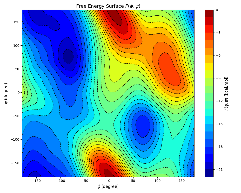
You can find several free energy minima and maxima on the FES.

Example: Proton Transfer of Malonaldehyde

Here we consider the following proton transfer reaction of malonaldehyde:

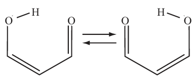
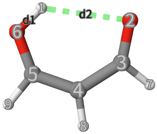
In you just do a standard MD, you may never see a protron transfering to another oxygen atom. To sample this rare event, we will use metadynamics. The intial structure is shown below. A nature set of CVs to describe the proton transfer is the 2 OH distances, but in this case, we want to plot a one-dimensional FES, so we will use the difference between the 2 distances \(d\equivd_1-d_2\):

The input file is:

malonaldehyde.inp

mol
    H      2.60849612     -0.72353966      0.29921536
    O      1.96497994     -0.12074426     -0.17095304
    C      2.66761718      0.78172105     -0.81146959
    C      4.02335932      0.83968127     -0.80715851
    C      4.77421680     -0.12520070     -0.05714631
    O      4.27344987     -1.03185159      0.59780685
    H      2.06272652      1.49828618     -1.35825644
    H      4.54176858      1.60740187     -1.35230520
    H      5.86993567     -0.01026417     -0.09028312
end

md
    type              NVT      # Type: NVE, NVT
    dt                0.001    # The time step in ps.
    temp              300.     # The temperature in Kelvin.
    temp_nhc_length   5        # The length of temperature Nose-Hoover chain.
    temp_nhc_tau      0.2      # The time constant of temperature Nose-Hoover chain in ps.
    num_steps         1000000  # The number of steps: 1 ns
    output_freq       1000     # The output frequency: 1 ps
    plumed_fn         plumed.dat
end

task
    md xtb
end

So, this will be a 10-ns NVT metadynamics using xTB, since only quantum chemistry can describe chemical reactions. xTB is fast, but less accurate than DFT.

The Plumed setting is shown below:

plumed.dat

# Compute the OH distances
d1: DISTANCE ATOMS=1,2
d2: DISTANCE ATOMS=1,6
d21: COMBINE ARG=d1,d2 COEFFICIENTS=1,-1 PERIODIC=NO

metad: METAD ...
   ARG=d21
   SIGMA=0.05
   HEIGHT=0.1
   PACE=100
   FILE=HILLS
   GRID_MIN=-0.5
   GRID_MAX=+0.5
...

# Print both collective variables on COLVAR file every 10 steps
PRINT ARG=d1,d2,d21 FILE=COLVAR STRIDE=10

Most settings have already been explained in the last exmaple. Just a few points:

• Line 2: Define the CV as distance between atom 1 and 2 named d1 using the keyword DISTANCE.

• Line 3: Similar to Line 2, but define the CV as distance between atom 1 and 6 named d2.

• Line 4: COMBINE is used to combine the two CVs, whose operation is d1` times 1 + d2 times -1.

Others should be self-explanatory. Now you can run the calculation.

Before calculating the FES, we can visualize the trajectory using malonaldehyde-md-traj.xyz in Qbics-MolStar:

We can see several proton transfer events between the 2 oxygen atoms. Without bias potentials from metadynamics, this is very difficult to happen.

Now, calculate the FES using the following command:

plumed sum_hills --hills HILLS

This will generate the file fes.dat. With the following Python script, we can plot the FES \(F(d)\):

plot_fes.py

Below is the FES plot:

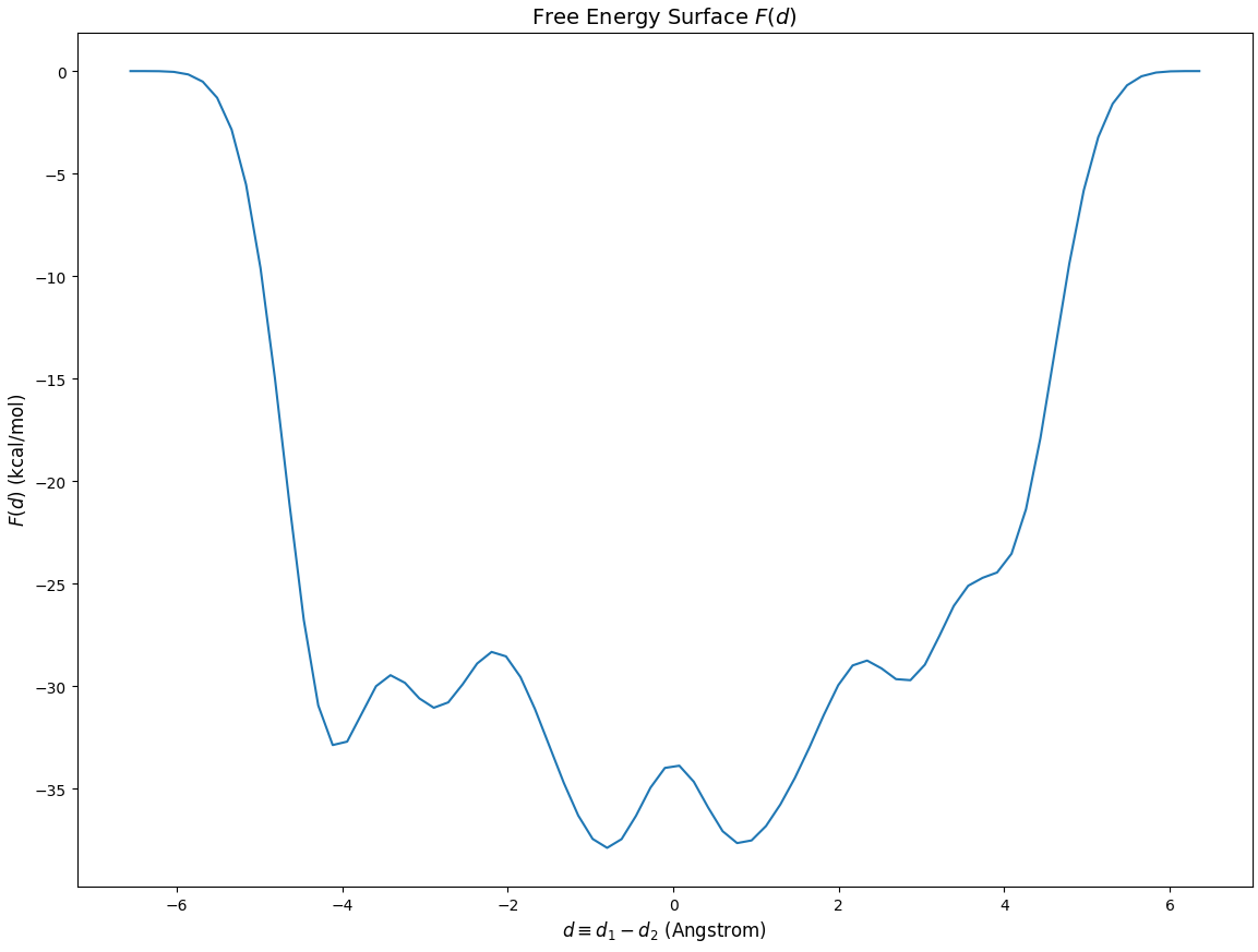
Although there are many local minima, we focus on the transfer region, which is [-1,1] Angstrom:

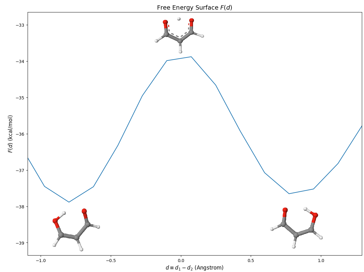
We show some representative structures in the picuture.

Fiinally, there are 3 points:

• The FES should be symmetric, but it is not. This is because the calculation is not completely converged.

• The xTB FES is not accurate. One should use DFT to get a more accurate FES in production research.

• One can add some restraints in plumed.dat to let \(d\) stay in [-1,1] during the metadynamics, but this needs an unbiasing/reweighting process to modify the FES, which is not discussed in this tutorial and can reter to Plumed documentation.