Tip
All input files can be downloaded: Files.
Tip
For more information of this section, please refer to these pages:
MSDFT (1): All Types of Excited States
This tutorial will lead you step by step to study excited states using Multi-State Density Functional Theory (MSDFT).
MSDFT is a powerful method for studying excited states. It optimizes excited states using TSO-DFT method, so it is free of orbital relaxation problem like in TDDFT. In this section, you will see that MSDFT can give much more reasonable results than TDDFT for excited states.
In TSO-DFT (1): Excited States, we have introduced how to use TSO-DFT to study excited states. Actually, MSDFT can be considered as TSO+NOSI. MSDFT is a framework that automaitcally performs TSO-DFT and NOSI for required excited states. Of course, you can also perform TSO-DFT and NOSI separately for special purposes.
Example: Broadspectrum for HCHO
HCHO is a typical molecule for studying excited states. As we know, HCHO has 8 occupied molecular orbitals (MOs), 2 of which are core orbitals (1s orbitals of carbon and oxygen atoms), and the remaining 6 are valence orbitals. Therefore, the excited states of HCHO to low-lying virtual orbitals contains 3 types: O K-edge excitation (O(1s) excitation), C K-edge excitation (C(1s) excitation), and valence excitations. TDDFT can show good performance for valence excitations, but it has errors for O and C K-edge excitations as large as 11 eV! A very important point is that MSDFT is balanced for all these 3 types of excitations, so in this example, we will use MSDFT to study all these 3 types of excitations of HCHO.
The input file is:
 1basis
 2    cc-pvtz
 3end
 4
 5scf
 6    charge  0
 7    spin2p1 1
 8    type    U
 9    schwarz 1E-14
10end
11
12msdft
13    single_ex 1-8 : 9-14
14end
15
16mol
17    O     -0.68710791      0.04339108      0.00000000
18    C      0.50595906     -0.07524732      0.00000008
19    H      1.09294418     -0.13258299     -0.93605972
20    H      1.09294415     -0.13258317      0.93605964
21end
22
23task
24    msdft b3lyp
25end
We explain the input file step by step:
basis...endindicates the basis set to be used. Here, we use cc-pvtz basis set.scf...endNote that we givetype Usince MSDFT must be run in unrestricted formalism.msdft...endindicates the MSDFT calculation. Here,single_ex 1-8 : 9-14means we want to study the single excitation from orbitals 1 to 8 and to orbitals 9 to 14. Explicitly, we want to study the following single excitations:1 → 9
2 → 9
3 → 9
4 → 9
5 → 9
6 → 9
7 → 9
8 → 9
1 → 10
2 → 10
3 → 10
4 → 10
5 → 10
6 → 10
7 → 10
8 → 10
…
1 → 14
2 → 14
3 → 14
4 → 14
5 → 14
6 → 14
7 → 14
8 → 14
So, single_ex 1-8 : 9-14 should be very self-explaining. After running this calculation, you will find the following output files:
hcho-1-to-10-se.mwfn  hcho-2-to-11-t.mwfn   hcho-3-to-13-se.mwfn  hcho-4-to-14-t.mwfn   hcho-6-to-10-se.mwfn  hcho-7-to-11-t.mwfn   hcho-8-to-13-se.mwfn
hcho-1-to-10-t.mwfn   hcho-2-to-12-se.mwfn  hcho-3-to-13-t.mwfn   hcho-4-to-9-se.mwfn   hcho-6-to-10-t.mwfn   hcho-7-to-12-se.mwfn  hcho-8-to-13-t.mwfn
hcho-1-to-11-se.mwfn  hcho-2-to-12-t.mwfn   hcho-3-to-14-se.mwfn  hcho-4-to-9-t.mwfn    hcho-6-to-11-se.mwfn  hcho-7-to-12-t.mwfn   hcho-8-to-14-se.mwfn
hcho-1-to-11-t.mwfn   hcho-2-to-13-se.mwfn  hcho-3-to-14-t.mwfn   hcho-5-to-10-se.mwfn  hcho-6-to-11-t.mwfn   hcho-7-to-13-se.mwfn  hcho-8-to-14-t.mwfn
hcho-1-to-12-se.mwfn  hcho-2-to-13-t.mwfn   hcho-3-to-9-se.mwfn   hcho-5-to-10-t.mwfn   hcho-6-to-12-se.mwfn  hcho-7-to-13-t.mwfn   hcho-8-to-9-se.mwfn
hcho-1-to-12-t.mwfn   hcho-2-to-14-se.mwfn  hcho-3-to-9-t.mwfn    hcho-5-to-11-se.mwfn  hcho-6-to-12-t.mwfn   hcho-7-to-14-se.mwfn  hcho-ci.txt
hcho-1-to-13-se.mwfn  hcho-2-to-14-t.mwfn   hcho-4-to-10-se.mwfn  hcho-5-to-11-t.mwfn   hcho-6-to-13-se.mwfn  hcho-7-to-14-t.mwfn   hcho-gs.mwfn
hcho-1-to-13-t.mwfn   hcho-2-to-9-se.mwfn   hcho-4-to-10-t.mwfn   hcho-5-to-12-se.mwfn  hcho-6-to-13-t.mwfn   hcho-7-to-9-se.mwfn   hcho.inp
hcho-1-to-14-se.mwfn  hcho-2-to-9-t.mwfn    hcho-4-to-11-se.mwfn  hcho-5-to-12-t.mwfn   hcho-6-to-14-se.mwfn  hcho-7-to-9-t.mwfn    hcho.mwfn
hcho-1-to-14-t.mwfn   hcho-3-to-10-se.mwfn  hcho-4-to-11-t.mwfn   hcho-5-to-13-se.mwfn  hcho-6-to-14-t.mwfn   hcho-8-to-10-se.mwfn  hcho.out
hcho-1-to-9-se.mwfn   hcho-3-to-10-t.mwfn   hcho-4-to-12-se.mwfn  hcho-5-to-13-t.mwfn   hcho-6-to-9-se.mwfn   hcho-8-to-10-t.mwfn   hcho-spectrum.txt
hcho-1-to-9-t.mwfn    hcho-3-to-11-se.mwfn  hcho-4-to-12-t.mwfn   hcho-5-to-14-se.mwfn  hcho-6-to-9-t.mwfn    hcho-8-to-11-se.mwfn  hcho-ts.mwfn
hcho-2-to-10-se.mwfn  hcho-3-to-11-t.mwfn   hcho-4-to-13-se.mwfn  hcho-5-to-14-t.mwfn   hcho-7-to-10-se.mwfn  hcho-8-to-11-t.mwfn
hcho-2-to-10-t.mwfn   hcho-3-to-12-se.mwfn  hcho-4-to-13-t.mwfn   hcho-5-to-9-se.mwfn   hcho-7-to-10-t.mwfn   hcho-8-to-12-se.mwfn
hcho-2-to-11-se.mwfn  hcho-3-to-12-t.mwfn   hcho-4-to-14-se.mwfn  hcho-5-to-9-t.mwfn    hcho-7-to-11-se.mwfn  hcho-8-to-12-t.mwfn
The meaning of these files should be very self-explaining:
hcho-1-to-10-se.mwfn: Singlet single excitation determinant from orbital 1 to 10. Calculated by TSO-DFT.hcho-1-to-10-t.mwfn: Triplet single excitation determinant from orbital 1 to 10. Calculated by TSO-DFT.hcho-gs.mwfn: Ground state determinant.hcho-ci.txt`: Configuration interaction (CI) coefficients between the ground state and the excited states.hcho-spectrum.txt: Excited state energies and oscillator strengths. It can be used to plot the spectrum.
A very good feature of MSDFT module in Qbics is that it can be restarted from the previous calculation. For example, with hcho.inp, if your calculation is interrupted, you can restart it from the previous calculation by simply running qbics hcho.inp again. Excited states that have been computed will not be calculated again.
In hcho-ci.txt, you will find the following information:
1hcho-gs.mwfn  hcho-1-to-9-se.mwfn  spin_flip_hcho-1-to-9-se.mwfn  hcho-1-to-10-se.mwfn  spin_flip_hcho-1-to-10-se.mwfn  hcho-1-to-11-se.mwfn  spin_flip_hcho-1-to-11-se.mwfn  hcho-1-to-12-se.mwfn  spin_flip_hcho-1-to-12-se.mwfn  hcho-1-to-13-se.mwfn  spin_flip_hcho-1-to-13-se.mwfn  hcho-1-to-14-se.mwfn  spin_flip_hcho-1-to-14-se.mwfn  hcho-2-to-9-se.mwfn  spin_flip_hcho-2-to-9-se.mwfn  hcho-2-to-10-se.mwfn  spin_flip_hcho-2-to-10-se.mwfn  hcho-2-to-11-se.mwfn  spin_flip_hcho-2-to-11-se.mwfn  hcho-2-to-12-se.mwfn  spin_flip_hcho-2-to-12-se.mwfn  hcho-2-to-13-se.mwfn  spin_flip_hcho-2-to-13-se.mwfn  hcho-2-to-14-se.mwfn  spin_flip_hcho-2-to-14-se.mwfn  hcho-3-to-9-se.mwfn  spin_flip_hcho-3-to-9-se.mwfn  hcho-3-to-10-se.mwfn  spin_flip_hcho-3-to-10-se.mwfn  hcho-3-to-11-se.mwfn  spin_flip_hcho-3-to-11-se.mwfn  hcho-3-to-12-se.mwfn  spin_flip_hcho-3-to-12-se.mwfn  hcho-3-to-13-se.mwfn  spin_flip_hcho-3-to-13-se.mwfn  hcho-3-to-14-se.mwfn  spin_flip_hcho-3-to-14-se.mwfn  hcho-4-to-9-se.mwfn  spin_flip_hcho-4-to-9-se.mwfn  hcho-4-to-10-se.mwfn  spin_flip_hcho-4-to-10-se.mwfn  hcho-4-to-11-se.mwfn  spin_flip_hcho-4-to-11-se.mwfn  hcho-4-to-12-se.mwfn  spin_flip_hcho-4-to-12-se.mwfn  hcho-4-to-13-se.mwfn  spin_flip_hcho-4-to-13-se.mwfn  hcho-4-to-14-se.mwfn  spin_flip_hcho-4-to-14-se.mwfn  hcho-5-to-9-se.mwfn  spin_flip_hcho-5-to-9-se.mwfn  hcho-5-to-10-se.mwfn  spin_flip_hcho-5-to-10-se.mwfn  hcho-5-to-11-se.mwfn  spin_flip_hcho-5-to-11-se.mwfn  hcho-5-to-12-se.mwfn  spin_flip_hcho-5-to-12-se.mwfn  hcho-5-to-13-se.mwfn  spin_flip_hcho-5-to-13-se.mwfn  hcho-5-to-14-se.mwfn  spin_flip_hcho-5-to-14-se.mwfn  hcho-6-to-9-se.mwfn  spin_flip_hcho-6-to-9-se.mwfn  hcho-6-to-10-se.mwfn  spin_flip_hcho-6-to-10-se.mwfn  hcho-6-to-11-se.mwfn  spin_flip_hcho-6-to-11-se.mwfn  hcho-6-to-12-se.mwfn  spin_flip_hcho-6-to-12-se.mwfn  hcho-6-to-13-se.mwfn  spin_flip_hcho-6-to-13-se.mwfn  hcho-6-to-14-se.mwfn  spin_flip_hcho-6-to-14-se.mwfn  hcho-7-to-9-se.mwfn  spin_flip_hcho-7-to-9-se.mwfn  hcho-7-to-10-se.mwfn  spin_flip_hcho-7-to-10-se.mwfn  hcho-7-to-11-se.mwfn  spin_flip_hcho-7-to-11-se.mwfn  hcho-7-to-12-se.mwfn  spin_flip_hcho-7-to-12-se.mwfn  hcho-7-to-13-se.mwfn  spin_flip_hcho-7-to-13-se.mwfn  hcho-7-to-14-se.mwfn  spin_flip_hcho-7-to-14-se.mwfn  hcho-8-to-9-se.mwfn  spin_flip_hcho-8-to-9-se.mwfn  hcho-8-to-10-se.mwfn  spin_flip_hcho-8-to-10-se.mwfn  hcho-8-to-11-se.mwfn  spin_flip_hcho-8-to-11-se.mwfn  hcho-8-to-12-se.mwfn  spin_flip_hcho-8-to-12-se.mwfn  hcho-8-to-13-se.mwfn  spin_flip_hcho-8-to-13-se.mwfn  hcho-8-to-14-se.mwfn  spin_flip_hcho-8-to-14-se.mwfn
2 0.99560913     -0.00000003     -0.00000003      0.00001534      0.00001534      0.00114350      0.00114351     -0.00153370     -0.00153371      0.00000039      0.00000039     -0.00010346     -0.00010346      0.00000179      0.00000179     -0.00107255     -0.00107255     -0.00000000     -0.00000000     -0.00040710     -0.00040710     -0.00000037     -0.00000037      0.00043794      0.00043795     -0.00002795     -0.00002777     -0.00436908     -0.00436911      0.00000000      0.00000002      0.01424106      0.01424114     -0.00000857     -0.00000861      0.00301359      0.00301360      0.00003226      0.00003213     -0.02803909     -0.02803946     -0.00000004     -0.00000023     -0.00129582     -0.00129576      0.00003624      0.00003624      0.01310570      0.01310577     -0.00000017     -0.00000044      0.00000015      0.00000060      0.03456283      0.03456304     -0.00000004     -0.00000007      0.00000004      0.00000004      0.00000030      0.00000035      0.00010560      0.00010920      0.01482854      0.01482881      0.00000010      0.00000017     -0.00405550     -0.00405553     -0.00001639     -0.00001653      0.00200558      0.00200559     -0.03841319     -0.03841054     -0.00006055     -0.00006067      0.00000004      0.00000005      0.00004803      0.00004811      0.01584468      0.01584465      0.00000846      0.00000847      0.00000020      0.00000236     -0.00000058      0.00000053     -0.00159919     -0.00159946     -0.00000014     -0.00000008      0.00000002     -0.00000001     -0.00000035     -0.00000035
3 0.00000150     -0.00000000      0.00000000      0.00000000      0.00000000      0.00000000      0.00000000     -0.00000000     -0.00000000      0.00000000     -0.00000000     -0.00000000     -0.00000000     -0.00000000      0.00000000     -0.00000000     -0.00000000      0.00000020     -0.00000020     -0.00000000     -0.00000000      0.00000000     -0.00000000      0.00000000      0.00000000     -0.00000003      0.00000003     -0.00000001     -0.00000001     -0.00000069      0.00000069      0.00000000      0.00000004     -0.00000001      0.00000001     -0.00000000      0.00000001      0.00000040     -0.00000040      0.00000001     -0.00000012     -0.00003928      0.00003928     -0.00000002      0.00000002     -0.00000003      0.00000003      0.00000004      0.00000001      0.04484569     -0.04484569      0.00009137     -0.00009137      0.00000003      0.00000010      0.00003755     -0.00003755      0.00284210     -0.00284210      0.00000866     -0.00000866     -0.00000071      0.00000072     -0.00000002      0.00000008      0.00002182     -0.00002182     -0.00000001     -0.00000001      0.00000003     -0.00000003      0.00000001     -0.00000001      0.00000007     -0.00000025     -0.00000000      0.00000000     -0.00331372      0.00331372     -0.00000001      0.00000001     -0.00000002      0.00000008     -0.00000001      0.00000001      0.70584687     -0.70584687      0.00000690     -0.00000690      0.00000028     -0.00000027     -0.00004415      0.00004415     -0.00418456      0.00418456     -0.00001737      0.00001737
4 0.00000177      0.00000000      0.00000000      0.00000000      0.00000000      0.00000000      0.00000000     -0.00000000     -0.00000000     -0.00000000     -0.00000000     -0.00000000     -0.00000000      0.00000000      0.00000000     -0.00000000     -0.00000000     -0.00000005     -0.00000005     -0.00000000     -0.00000000     -0.00000000     -0.00000000      0.00000000      0.00000000      0.00000003      0.00000003     -0.00000001     -0.00000001      0.00000366      0.00000366      0.00000001      0.00000001      0.00000001      0.00000001      0.00000000      0.00000000     -0.00000040     -0.00000040     -0.00000004     -0.00000004      0.00001763      0.00001763     -0.00000003     -0.00000003      0.00000003      0.00000003      0.00000001      0.00000001     -0.05112536     -0.05112536     -0.00005166     -0.00005166      0.00000004      0.00000004     -0.00002375     -0.00002375     -0.00104504     -0.00104504      0.00002882      0.00002882      0.00000075      0.00000075     -0.00000000     -0.00000000     -0.00000653     -0.00000653     -0.00000001     -0.00000001     -0.00000003     -0.00000003      0.00000001      0.00000001     -0.00000006     -0.00000006      0.00000002      0.00000002      0.00094859      0.00094859     -0.00000001     -0.00000001     -0.00000001     -0.00000001     -0.00000001     -0.00000001     -0.70546067     -0.70546067     -0.00005036     -0.00005036     -0.00000010     -0.00000010      0.00002947      0.00002947      0.00517794      0.00517794     -0.00002117     -0.00002117
5-0.00000008      0.00000014     -0.00000014      0.00000064     -0.00000064     -0.00053975      0.00053975      0.00086019     -0.00086019     -0.00000038      0.00000038      0.00008698     -0.00008698      0.00000187     -0.00000187     -0.00047589      0.00047589     -0.00000000      0.00000000     -0.00027619      0.00027619      0.00000007     -0.00000007      0.00031214     -0.00031214      0.00001230     -0.00001230      0.00800444     -0.00800444     -0.00000001      0.00000001     -0.01812879      0.01812879      0.00001604     -0.00001604     -0.01082709      0.01082709     -0.00011444      0.00011444     -0.02131200      0.02131201      0.00000004     -0.00000004      0.00193396     -0.00193396     -0.00000881      0.00000881      0.01598192     -0.01598192     -0.00000044      0.00000044     -0.00000007      0.00000007      0.01268254     -0.01268254     -0.00000002      0.00000002     -0.00000001      0.00000001     -0.00000002      0.00000002     -0.00036683      0.00036683     -0.00437980      0.00437980     -0.00000005      0.00000005      0.00068293     -0.00068293     -0.00000034      0.00000034      0.00219123     -0.00219123      0.71248403     -0.71248402      0.00005779     -0.00005779     -0.00000013      0.00000013      0.00023606     -0.00023606      0.00112889     -0.00112889      0.00006985     -0.00006985     -0.00000013      0.00000013      0.00000035     -0.00000035     -0.00251385      0.00251385      0.00000004     -0.00000004     -0.00000001      0.00000001      0.00000005     -0.00000005
6...
Each line is a state with coefficients. They are the same with the following lines in hcho.out, but are more convienent for automatic analysis:
 1---- NOSI Coefficients Matrix (column vectors are eigenvectors) ----
 2====================================================================
 3                  0              1              2              3              4
 4   0     0.99560913     0.00000150     0.00000177    -0.00000008     0.00000018
 5   1    -0.00000003    -0.00000000     0.00000000     0.00000014     0.00000000
 6   2    -0.00000003     0.00000000     0.00000000    -0.00000014     0.00000000
 7   3     0.00001534     0.00000000     0.00000000     0.00000064    -0.00000000
 8   4     0.00001534     0.00000000     0.00000000    -0.00000064     0.00000000
 9   5     0.00114350     0.00000000     0.00000000    -0.00053975     0.00000004
10   6     0.00114351     0.00000000     0.00000000     0.00053975    -0.00000004
11   7    -0.00153370    -0.00000000    -0.00000000     0.00086019    -0.00000004
12   8    -0.00153371    -0.00000000    -0.00000000    -0.00086019     0.00000004
13   9     0.00000039     0.00000000    -0.00000000    -0.00000038     0.00000000
14  10     0.00000039    -0.00000000    -0.00000000     0.00000038    -0.00000000
15  11    -0.00010346    -0.00000000    -0.00000000     0.00008698     0.00000000
16  12    -0.00010346    -0.00000000    -0.00000000    -0.00008698    -0.00000000
17  13     0.00000179    -0.00000000     0.00000000     0.00000187     0.00000000
18  14     0.00000179     0.00000000     0.00000000    -0.00000187    -0.00000000
19  15    -0.00107255    -0.00000000    -0.00000000    -0.00047589     0.00000000
The following lines are excitation energies and oscillator strengths, which are also in hcho-spectrum.txt:
 1---- NOSI Results ----
 2======================
 3   State   NOSI Energies  Excited Energy       Osc. Str.        DX        DY        DZ
 4               (Hartree)            (eV)                    (a.u.)    (a.u.)    (a.u.)
 5       0   -114.55472122      0.00000000      0.00000000  -1.67410  -0.89631   0.00000
 6       1   -114.43192614      3.34125415      0.00000000   0.00000   0.00000   0.00000
 7       2   -114.41053475      3.92331383      0.00000004   0.00000   0.00000  -0.00088
 8       3   -114.39885445      4.24113491      0.00000000  -0.00000   0.00000  -0.00000
 9       4   -114.27926662      7.49511958      0.00000000   0.00000  -0.00000  -0.00000
10       5   -114.26311475      7.93461209      0.00000000   0.00000  -0.00000   0.00000
11       6   -114.26115827      7.98784791      0.10048800   0.00000  -0.00000  -1.01488
12       7   -114.23545182      8.68732031      0.00000000  -0.00000   0.00000   0.00000
13       8   -114.22993229      8.83750667      0.00148189   0.01385   0.11635   0.00000
14       9   -114.22276183      9.03261499      0.00171129  -0.12377   0.01390  -0.00000
15      10   -114.20424336      9.53650263      0.00000000  -0.00000  -0.00000   0.00000
16      11   -114.20235213      9.58796291      0.00000000  -0.00000   0.00000  -0.00000
17      12   -114.18660197     10.01652481      0.03607540   0.00000   0.00000  -0.54302
18      13   -114.17489121     10.33517463      0.00000022   0.00000   0.00000  -0.00132
The following lines list the states and their high-weighted Slater determinants:
 1---- NOSI State Identification (Coefficients) ----
 2==================================================
 3State |0> = +0.996 |hcho-gs.mwfn>
 4State |1> = +0.706 |hcho-8-to-9-se.mwfn> -0.706 |spin_flip_hcho-8-to-9-se.mwfn>
 5State |2> = -0.705 |hcho-8-to-9-se.mwfn> -0.705 |spin_flip_hcho-8-to-9-se.mwfn>
 6State |3> = +0.712 |hcho-7-to-9-se.mwfn> -0.712 |spin_flip_hcho-7-to-9-se.mwfn>
 7State |4> = -0.700 |hcho-8-to-10-se.mwfn> +0.700 |spin_flip_hcho-8-to-10-se.mwfn>
 8State |5> = +0.703 |hcho-6-to-9-se.mwfn> -0.703 |spin_flip_hcho-6-to-9-se.mwfn>
 9State |6> = +0.704 |hcho-8-to-10-se.mwfn> +0.704 |spin_flip_hcho-8-to-10-se.mwfn>
10State |7> = -0.695 |hcho-8-to-11-se.mwfn> +0.695 |spin_flip_hcho-8-to-11-se.mwfn>
11...
12
13---- NOSI State Identification (Weights) ----
14=============================================
15State |0> = 0.991 |hcho-gs.mwfn>
16State |1> = 0.498 |hcho-8-to-9-se.mwfn> 0.498 |spin_flip_hcho-8-to-9-se.mwfn>
17State |2> = 0.498 |hcho-8-to-9-se.mwfn> 0.498 |spin_flip_hcho-8-to-9-se.mwfn>
18State |3> = 0.499 |hcho-7-to-9-se.mwfn> 0.499 |spin_flip_hcho-7-to-9-se.mwfn>
19State |4> = 0.489 |hcho-8-to-10-se.mwfn> 0.489 |spin_flip_hcho-8-to-10-se.mwfn>
20State |5> = 0.495 |hcho-6-to-9-se.mwfn> 0.495 |spin_flip_hcho-6-to-9-se.mwfn>
21State |6> = 0.495 |hcho-8-to-10-se.mwfn> 0.495 |spin_flip_hcho-8-to-10-se.mwfn>
22State |7> = 0.480 |hcho-8-to-11-se.mwfn> 0.480 |spin_flip_hcho-8-to-11-se.mwfn>
From these, we can know that the state 0 is the ground state, and the state 1 and 2 are mainly composed of the excited state of MO 8 → 9. Note that if the coefficients are of the opposite sign, then it is a triplet state; if the coefficients are of the same sign, then it is a singlet state., so state 1 is triplet 8 → 9 excitated state; state 2 is singlet 8 → 9 excitated state. Then, state 3 is triplet 7 → 9 excitated state; state 4 is triplet 8 → 10 excitated state; state 5 is triplet 6 → 9 excitated state; state 6 is singlet 8 → 10 excitated state; state 7 is triplet 8 → 11 excitated state, and so on.
With hcho-spectrum.txt, we can plot the spectrum of the molecule using the python script provided in qbics/tools/plotspec.py. Copy it to the same directory as hcho-spectrum.txt, and modify the following parameters:
1if __name__ == "__main__":
2    fn = "hcho-spectrum.txt" # Spectrum file name.
3    eL_eV = 3.3                 # Lower energy limit.
4    eH_eV = 558.6                 # Higher energy limit.
5    sigma_eV = 0.2              # Sigma value.
6    num_ps = 3000                # Number of points.
7    use_angle = False           # Whether to use angle dependence.
Tip
Please cite this paper, if you use this script and formular in it:
Here, we want to plot the spectrum from 3.3 (eL_eV) to 558.6 (eH_eV) eV, with a sigma value of 0.2 (sigma_eV) and 3000 (num_ps) points. Run ./plotspec.py to get the spectrum plot:
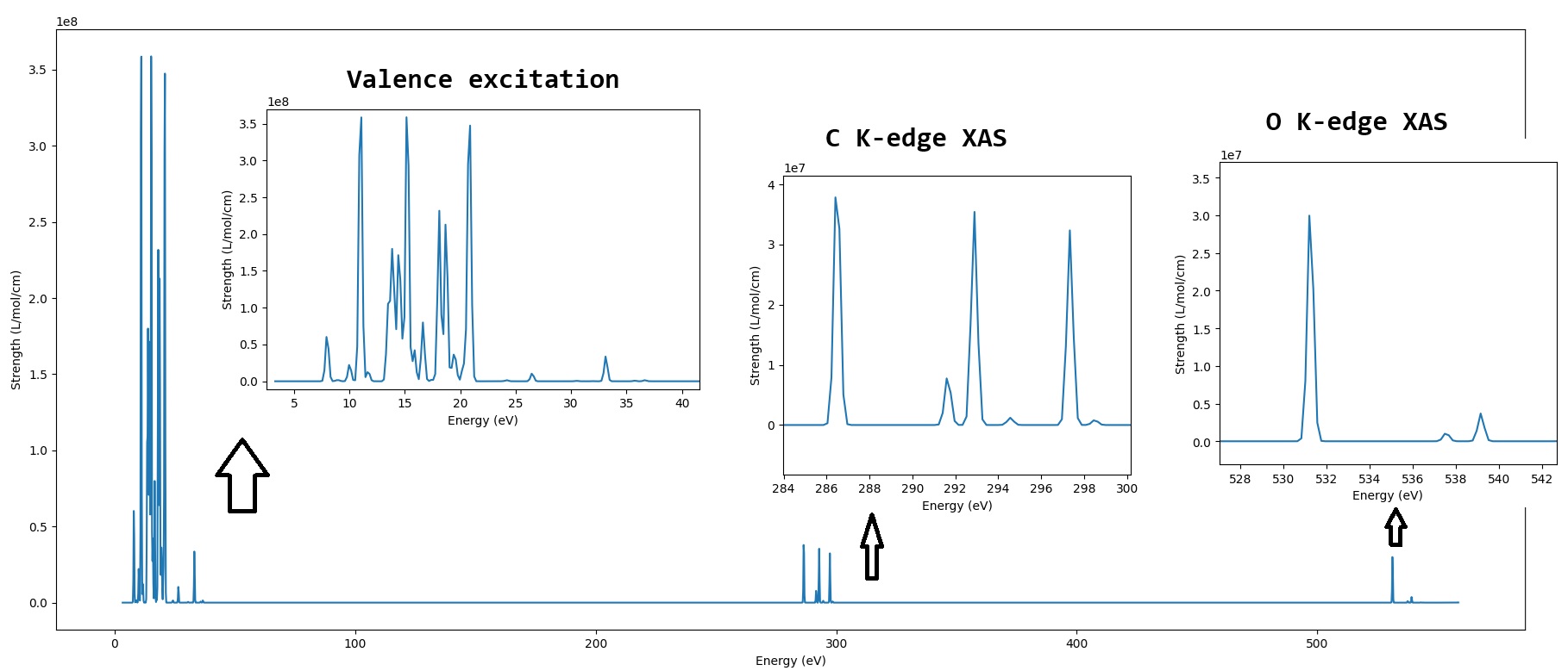
We can see that, MSDFT can plot broadspectrum, ranging from 3.3 eV to 558.6 eV, including valence and core excitations.
Example: Valence Excitations for HCHO
Of course, we can use MSDFT to plot only a part of the spectrum. For example, we can only calculate valence excitations, MO 8 → 9 (HOMO → LUMO) and MO 8 → 10 (HOMO → LUMO+1). So use the following input file:
 1basis
 2    cc-pvtz
 3end
 4
 5scf
 6    charge  0
 7    spin2p1 1
 8    type    U
 9    schwarz 1E-14
10end
11
12msdft
13    single_ex 8 : 9 10
14end
15
16mol
17    O     -0.68710791      0.04339108      0.00000000
18    C      0.50595906     -0.07524732      0.00000008
19    H      1.09294418     -0.13258299     -0.93605972
20    H      1.09294415     -0.13258317      0.93605964
21end
22
23task
24    msdft b3lyp
25end
The output is:
 1---- NOSI Results ----
 2======================
 3   State   NOSI Energies  Excited Energy       Osc. Str.        DX        DY        DZ
 4               (Hartree)            (eV)                    (a.u.)    (a.u.)    (a.u.)
 5       0   -114.54951400      0.00000000      0.00000000  -2.00272  -0.86383   0.00000
 6       1   -114.43098101      3.22528264      0.00000000   0.00001  -0.00000   0.00000
 7       2   -114.40928299      3.81568579      0.00000003   0.00005  -0.00001   0.00080
 8       3   -114.27311171      7.52090618      0.00000000  -0.00000  -0.00000   0.00000
 9       4   -114.25847627      7.91913672      0.12823740  -0.00000   0.00000   1.15144
10
11---- NOSI State Identification (Coefficients) ----
12==================================================
13State |0> = -1.000 |valence-gs.mwfn>
14State |1> = +0.707 |valence-8-to-9-se.mwfn> -0.707 |spin_flip_valence-8-to-9-se.mwfn>
15State |2> = +0.707 |valence-8-to-9-se.mwfn> +0.707 |spin_flip_valence-8-to-9-se.mwfn>
16State |3> = -0.707 |valence-8-to-10-se.mwfn> +0.707 |spin_flip_valence-8-to-10-se.mwfn>
17State |4> = +0.707 |valence-8-to-10-se.mwfn> +0.707 |spin_flip_valence-8-to-10-se.mwfn>
18
19---- NOSI State Identification (Weights) ----
20=============================================
21State |0> = 1.000 |valence-gs.mwfn>
22State |1> = 0.500 |valence-8-to-9-se.mwfn> 0.500 |spin_flip_valence-8-to-9-se.mwfn>
23State |2> = 0.500 |valence-8-to-9-se.mwfn> 0.500 |spin_flip_valence-8-to-9-se.mwfn>
24State |3> = 0.500 |valence-8-to-10-se.mwfn> 0.500 |spin_flip_valence-8-to-10-se.mwfn>
25State |4> = 0.500 |valence-8-to-10-se.mwfn> 0.500 |spin_flip_valence-8-to-10-se.mwfn>
The 5 states are: 0 is the ground state, 1 and 2 are the triplet and singlet excited state of MO 8 → 9, respectively; 3 and 4 are the triplet and singlet excited state of MO 8 → 10, respectively.