Tip
All input files can be downloaded: Files.
Tip
For detailed tutorials of MSDFT, please refer to the following ones:
msdft
This option defines the implementation details of multi-state density functional theory (MSDFT) for excited and diabaitc states.
- offdiag_correlation
Value
overlap_weightedWill use overlap weighted methodenergy_weightedWill use energy weighted methodcorrelation_potentialWill use correlation functional method, given by thexc_functionaloptionDefault
overlap_weightedDefine the off-diagonal correlation method.
- single_ex
Value
Single excitations to be considered
Default
None
This option indicates what single excitations are considered.
The input format is:
single_ex occupied_MO_incides : virtual_MO_indicesFor example,
single_ex 1 5-6 9 : 10-13 15considers the following single excitations:1 → 10
1 → 11
1 → 13
1 → 15
5 → 10
5 → 11
5 → 13
5 → 15
6 → 10
6 → 11
6 → 13
6 → 15
9 → 10
9 → 11
9 → 13
9 → 15
- double_ex
Value
Double excitations to be considered
Default
None
This option indicates what double excitations are considered.
The input format is:
double_ex occupied_MO_incides : virtual_MO_indicesFor example,
double_ex 1 5-6 9 : 10-13 15considers the following double excitations:1 → 10
1 → 11
1 → 13
1 → 15
5 → 10
5 → 11
5 → 13
5 → 15
6 → 10
6 → 11
6 → 13
6 → 15
9 → 10
9 → 11
9 → 13
9 → 15
Theoretical Background
XXXXXX
Input Examples
Tip
For detailed tutorials of MSDFT, please refer to the following ones:
Example: Excited States of (E)-Dimethyldiazene (Automatically)
In this example, we will calculate the ground state and 2 singlet excited states of (E)-Dimethyldiazene with MSDFT methods. We will use B3LYP/cc-pVTZ level of theory.
Tip
Acutally, in Qbics, the calculation of excited states using MSDFT is close to (but NOT the same as) TSO+NOSI. See scfguess and nosi for details.
The input file is:
 1basis
 2    cc-pvtz
 3end
 4
 5scf
 6    charge      0
 7    spin2p1     1
 8    type        U
 9end
10
11mol
12    N     -0.11855722      0.06367877     -0.00010027
13    N      1.11855814     -0.06366086     -0.00010026
14    C      1.81864333      1.22402113      0.00009549
15    H      1.12816980      2.07452976      0.00011126
16    H      2.46787129      1.25512096      0.88302715
17    H      2.46820089      1.25538193     -0.88260363
18    C     -0.81864582     -1.22402070      0.00009559
19    H     -0.12816015     -2.07453667      0.00011125
20    H     -1.46787530     -1.25512668      0.88303320
21    H     -1.46820496     -1.25538766     -0.88260977
22end
23
24msdft
25    single_ex 15 16 : 17
26end
27
28task
29    msdft b3lyp
30end
Here, single_ex 15 16 : 17 indicates that 1 electron in the 15th or 16th MO is excited to the 17th MO, i.e.:
15 → 17
16 → 17
In msdft...end, there is no offdiag_correlation option. This means that the off-diagonal correlation will be calculated using the (default) overlap weighted method.
After calculation, we will obtain the output file msdft-1.out and wavefunction files msdft-1-gs.mwfn, msdft-1-15-to-17-se.mwfn, msdft-1-16-to-17-se.mwfn. etc. Their names are self-explaining. For example, msdft-1-15-to-17-se.mwfn is the wavefunction file for the single excitation from 15th to 17th MO.
In the output file msdft-1.out, we can find the following information:
 1Read non-orthogonal determinants:
 20 msdft-1-gs.mwfn
 31 msdft-1-15-to-17-se.mwfn
 4Spin flipped: msdft-1-15-to-17-se.mwfn
 52 msdft-1-16-to-17-se.mwfn
 6Spin flipped: msdft-1-16-to-17-se.mwfn
 7
 8---- NOSI Overlap Matrix ----
 9=============================
10                  0              1              2              3              4
11   0     1.00000000     0.00000000     0.00004807     0.00000000     0.00000778
12   1     0.00000000     1.00000000     0.00000000     0.00000000     0.00000000
13   2     0.00004807     0.00000000     1.00000000     0.00000000     0.00000000
14   3     0.00000000     0.00000000     0.00000000     1.00000000     0.00000000
15   4     0.00000778     0.00000000     0.00000000     0.00000000     1.00000000
16
17---- NO Hamiltonian Matrix Functional ----
18==========================================
19                  0              1              2              3              4
20   0  -189.34737100     0.00000019    -0.00909719    -0.00000028    -0.00147274
21   1     0.00000019  -189.11479500     0.09271220    -0.00000307    -0.00000741
22   2    -0.00909719     0.09271220  -189.11479500    -0.00000741    -0.00000307
23   3    -0.00000028    -0.00000307    -0.00000741  -189.24112500     0.02098466
24   4    -0.00147274    -0.00000741    -0.00000307     0.02098466  -189.24112500
25
26---- NOSI Coefficients Matrix (column vectors are eigenvectors) ----
27====================================================================
28                  0              1              2              3              4
29   0    -1.00000000    -0.00000085    -0.00000551    -0.00001218    -0.00002378
30   1    -0.00000820     0.00005595     0.00003731    -0.70710678     0.70710678
31   2     0.00002264    -0.00005595     0.00003731     0.70710678     0.70710678
32   3    -0.00000330    -0.70710678     0.70710678    -0.00005595    -0.00003731
33   4     0.00000328     0.70710678     0.70710678     0.00005595    -0.00003731
34
35---- Singlet and Triplet Excitation Energies ----
36=================================================
37Eigenstate 0: -189.34737100 Hartree; Excitation energy: 0.00000000 eV
38Eigenstate 1: -189.26210966 Hartree; Excitation energy: 2.32008047 eV
39Eigenstate 2: -189.22014034 Hartree; Excitation energy: 3.46212432 eV
40Eigenstate 3: -189.20750727 Hartree; Excitation energy: 3.80588786 eV
41Eigenstate 4: -189.02208273 Hartree; Excitation energy: 8.85154931 eV
42
43---- Singlet State Weights ----
44===============================
45                  0              1              2              3              4
46   0     1.00000000    -0.00000000     0.00000000    -0.00000000    -0.00000000
47   1     0.00000000     0.00000000     0.00000000     0.50000000     0.50000000
48   2    -0.00000000     0.00000000     0.00000000     0.50000000     0.50000000
49   3     0.00000000     0.50000000     0.50000000     0.00000000     0.00000000
50   4    -0.00000000     0.50000000     0.50000000     0.00000000     0.00000000
51
52---- NOSI Results ----
53======================
54   State   NOSI Energies  Excited Energy       Osc. Str.        DX        DY        DZ
55               (Hartree)            (eV)                    (a.u.)    (a.u.)    (a.u.)
56       0   -189.34737100      0.00000000      0.00000000  42.82334   0.00028   0.00212
57       1   -189.26210966      2.31996110      0.00000000   0.00000  -0.00000  -0.00001
58       2   -189.22014034      3.46194620      0.00000000  -0.00000   0.00005   0.00001
59       3   -189.20750727      3.80569205      0.00000000  -0.00000  -0.00000  -0.00000
60       4   -189.02208273      8.85109391      0.94030373   2.85146   0.75306   0.00000
In Read non-orthogonal determinants:, the determinants are shown:
\(\phi_0\) msdft-1-gs.mwfn
\(\phi_1\) msdft-1-15-to-17-se.mwfn
\(\phi_2\) msdft-1-15-to-17-se.mwfn (spin flipped)
\(\phi_3\) msdft-1-16-to-17-se.mwfn
\(\phi_4\) msdft-1-16-to-17-se.mwfn (spin flipped)
In NOSI Overlap Matrix, the matrix elements \(\left\langle\phi_i\middle|\phi_j\right\rangle\) are calculated.
In NO Hamiltonian Matrix Functional, the matrix elements \(\left\langle\phi_i\left|\hat{H}\right|\phi_j\right\rangle\) are calculated.
In NOSI Coefficients Matrix, the column vectors are eigenvectors of the NOSI Hamiltonian matrix. For example, in column 1, we have:
When a determinant and its spin flipped counterpart are combined with out-of-phases (-0.70710678 and -0.70710678), this is a triplet state. When a determinant and its spin flipped counterpart are combined with in-phases (0.70710678 and 0.70710678), this is a singlet state.
The excited energies are shown in NOSI Results.
A CI coefficient file and a spectrum file are generated. For example, msdft-1-ci.txt and msdft-1-spectrum.txt.
You can see that the energies are slightly different from the results obtained by TSO+NOSI in nosi. This is because the MSDFT method applied triplet correction, which should be more accurate.
State |
MSDFT (eV) |
TSO+NOSI (eV) (see nosi) |
S0 |
0.00000000 |
0.00000000 |
T1 |
2.31996110 |
2.32371833 |
S1 |
3.46194620 |
3.45818894 |
T2 |
3.80569205 |
3.82320418 |
S2 |
8.85109391 |
8.83363623 |
Example: N and O K-Edge XAS of N2O
In this example, we will calculate the K-edge XAS of N2O with MSDFT methods. We will use B3LYP/cc-pCVTZ level of theory. Here, “K-edge” means that the excitation is from 1s orbital to virtual ones. We use aug-cc-pCVTZ instead of aug-cc-pVTZ because the “pCVTZ” is highly optimized for core orbitals.
First, we do a standard SCF calculation for N:sub:`2`O to see orbitals. The input file is:
 1basis
 2    aug-cc-pCVTZ
 3end
 4
 5scf
 6    charge      0
 7    spin2p1     1
 8    type        U
 9end
10
11mol
12    N      0.     0.    -0.14168067
13    N      0.     0.     0.97956073
14    O      0.     0.     2.16211994
15end
16
17task
18    energy b3lyp
19end
Now we can visualize the molecular orbitals. Open Qbics-MolStar, and drag n2o-gs.mwfn into explorer, and it will be automatically loaded. Right-click n2o-gs.mwfn and select View Molecular Orbitals. Click the MOs and see below:
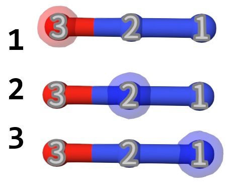
Obviously, the MO 1 is the 1s orbitals for oxygen, and the MO 2,3 are the 1s orbitals for nitrogen. The N and O K-edge XAS are quiet separated, so it is better (but not necessary) to calculate them separately with MSDFT methods. The input files for O and N K-edge XAS are:
 1basis
 2    aug-cc-pCVTZ
 3end
 4
 5scf
 6    charge      0
 7    spin2p1     1
 8    type        U
 9end
10
11mol
12    N      0.     0.    -0.14168067
13    N      0.     0.     0.97956073
14    O      0.     0.     2.16211994
15end
16
17msdft
18    single_ex 1 : 12-18
19end
20
21task
22    msdft b3lyp
23end
 1basis
 2    aug-cc-pCVTZ
 3end
 4
 5scf
 6    charge      0
 7    spin2p1     1
 8    type        U
 9end
10
11mol
12    N      0.     0.    -0.14168067
13    N      0.     0.     0.97956073
14    O      0.     0.     2.16211994
15end
16
17msdft
18    single_ex 2 3 : 12-18
19end
20
21task
22    msdft b3lyp
23end
Here, single_ex 1 : 12-18 indicates that 1 electron in the 1st MO is excited to the 12th to 18th MO; single_ex 2 3 : 12-18 indicates that 1 electron in the 2nd and 3rd MO is excited to the 12th to 18th MO. You can excite them to higher virtual MOs to get more accurate results.
After calculation, we will obtain the output files msdft-2-O.out and msdft-2-N.out. The excited state MWFN files are also available. There are also files for spertrum plotting: msdft-2-O-spectrum.txt and msdft-2-N-spectrum.txt.
For example, in msdft-2-N.out, we can find the following information:
 1---- NOSI Results ----
 2======================
 3   State   NOSI Energies  Excited Energy       Osc. Str.        DX        DY        DZ
 4               (Hartree)            (eV)                    (a.u.)    (a.u.)    (a.u.)
 5       0   -184.74191466      0.00000000      0.00000000  -0.00000   0.00001  62.02962
 6       1   -170.03989460    400.04196592      0.00000000   0.00000  -0.00000   0.00000
 7       2   -170.03502387    400.17449843      0.00000000  -0.00000   0.00000  -0.00000
 8       3   -170.01752034    400.65076950      0.05261600   0.06433   0.08133   0.00000
 9       4   -170.01547342    400.70646604      0.05144446   0.08040  -0.06362  -0.00000
10       5   -169.92447560    403.18251673      0.00000000   0.00000  -0.00000   0.00000
11       6   -169.91893969    403.33314900      0.00000000   0.00000  -0.00000  -0.00000
12       7   -169.91191435    403.52430858      0.00000000  -0.00000   0.00000   0.00000
13       8   -169.91076621    403.55554928      0.00534389   0.00000  -0.00000   0.03293
14       9   -169.88759854    404.18594177      0.06488836  -0.07104  -0.08999   0.00000
15      10   -169.88267696    404.31985772      0.06490275   0.08998  -0.07104   0.00000
16      11   -169.83564482    405.59960229      0.00000000  -0.00000  -0.00000   0.00000
17      12   -169.82950253    405.76673395      0.00925187  -0.00000   0.00000   0.04321
18      13   -169.81735744    406.09720202      0.00000000   0.00000   0.00000   0.00000
19      14   -169.81567589    406.14295698      0.00498163  -0.02593  -0.01821   0.00000
20      15   -169.81376836    406.19486083      0.00000000  -0.00000   0.00000  -0.00000
21      16   -169.81204070    406.24187047      0.00494890   0.01812  -0.02586   0.00000
22      17   -169.80681991    406.38392818      0.00000000  -0.00000  -0.00000   0.00000
23      18   -169.79772608    406.63137137      0.01209756   0.00000  -0.00000  -0.04935
24      19   -169.74853637    407.96982327      0.00000000  -0.00000   0.00000  -0.00000
25      20   -169.74401565    408.09283219      0.00113590   0.00000   0.00000   0.01510
26      21   -169.67330415    410.01689210      0.00000000   0.00000  -0.00000   0.00000
27      22   -169.67060344    410.09037844      0.00107912   0.00000  -0.00000  -0.01468
28      23   -169.65887737    410.40944479      0.00000000   0.00000  -0.00000   0.00000
29      24   -169.63235011    411.13125137      0.00601950   0.00000   0.00000  -0.03462
30      25   -169.07874371    426.19488170      0.00004203   0.00000  -0.00000  -0.00284
31      26   -169.07628789    426.26170433      0.00000000   0.00000   0.00000  -0.00000
32      27   -166.93991246    484.39247991      0.00003223  -0.00000  -0.00000   0.00233
33      28   -166.93767426    484.45338124      0.00000000   0.00000  -0.00000  -0.00000
You can identify the states from output files. For example, the coefficients of state 4 are:
 1---- NOSI Coefficients Matrix (column vectors are eigenvectors) ----
 2====================================================================
 3                  0              1              2              3              4
 4   0     0.99999900     0.00000000    -0.00000000     0.00000000    -0.00000000
 5   1    -0.00000000    -0.00573951    -0.00000102     0.00074472    -0.00000001
 6   2    -0.00000000     0.00573951     0.00000102     0.00074472    -0.00000001
 7   3    -0.00000000     0.00000132     0.00527620    -0.00000167    -0.00020742
 8   4    -0.00000000    -0.00000132    -0.00527620    -0.00000167    -0.00020742
 9   5    -0.00009224    -0.00000000     0.00000000     0.00000000    -0.00000000
10   6    -0.00009224     0.00000000    -0.00000000     0.00000000    -0.00000000
11   7    -0.00005050     0.00000004    -0.00000004    -0.00000003     0.00000003
12   8    -0.00005050    -0.00000004     0.00000004    -0.00000003     0.00000003
13   9    -0.01938433     0.00000002     0.00000006     0.00000027     0.00000011
14  10    -0.01938443    -0.00000002    -0.00000006     0.00000027     0.00000011
15  11    -0.01615554    -0.00000011     0.00000024    -0.00000053     0.00000224
16  12    -0.01615584     0.00000011    -0.00000024    -0.00000053     0.00000224
17  13    -0.00408296     0.00000017    -0.00000022     0.00000078    -0.00000210
18  14    -0.00408276    -0.00000017     0.00000022     0.00000078    -0.00000210
19  15     0.00000000     0.70440082     0.00016811    -0.70886826     0.00029439
20  16     0.00000000    -0.70440082    -0.00016811    -0.70886826     0.00029439
21  17     0.00000000     0.00007913    -0.70442320     0.00045204     0.70883620
22  18     0.00000000    -0.00007913     0.70442320     0.00045204     0.70883620
23  19    -0.00027387     0.00000004    -0.00000009    -0.00000007     0.00000003
24  20    -0.00027386    -0.00000004     0.00000009    -0.00000007     0.00000003
25  21    -0.00036762     0.00000357    -0.00000375    -0.00000369     0.00000380
26  22    -0.00036762    -0.00000357     0.00000376    -0.00000369     0.00000380
27  23    -0.00000001    -0.01231909    -0.00528893    -0.00894872    -0.00371633
28  24    -0.00000001     0.01231909     0.00528893    -0.00894872    -0.00371633
29  25     0.00000002     0.00424293    -0.01251586     0.00260869    -0.00878159
30  26     0.00000002    -0.00424293     0.01251586     0.00260869    -0.00878159
31  27     0.00040798    -0.00000375     0.00000392     0.00000362    -0.00000376
32  28     0.00040798     0.00000376    -0.00000392     0.00000362    -0.00000376
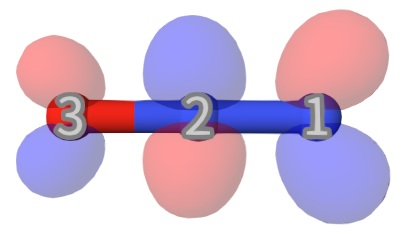
The largest coefficients for state 4 is \(0.70883620\phi_{17}+0.70883620\phi_{18}\), which is the combination of msdft-2-N-3-to-13-se.mwfn and its spin flipped one. So, this state is mainly the 3→13 single excitation, i.e. terminal-nitrogen \(1s\rightarrow\pi^*\) excitation (see below for MO 13, which is a \(\pi^*\) MO)
To plot the spectrum, you can use the script tools/plotspec.py provided by Qbics (or any tools you like). Assume you want to plot ```` First, copy this file to the same directory as the input file, and modify the following parameters:
1if __name__ == "__main__":
2    fn = "msdft-2-N-spectrum.txt" # Spectrum file name.
3    eL_eV = 400                 # Lower energy limit.
4    eH_eV = 410                 # Higher energy limit.
5    sigma_eV = 0.2              # Sigma value.
6    num_ps = 500                # Number of points.
7    use_angle = False           # Whether to use angle dependence.
Here, we want to plot the spectrum from 400 (eL_eV) to 410 (eH_eV) eV, with a sigma value of 0.2 (sigma_eV) and 500 (num_ps) points. You can change these parameters to get the desired spectrum.
Tip
Please cite this paper, if you use this script and formular in it:
The N and O K-edge XAS spectra as well as experimental data are shown below:
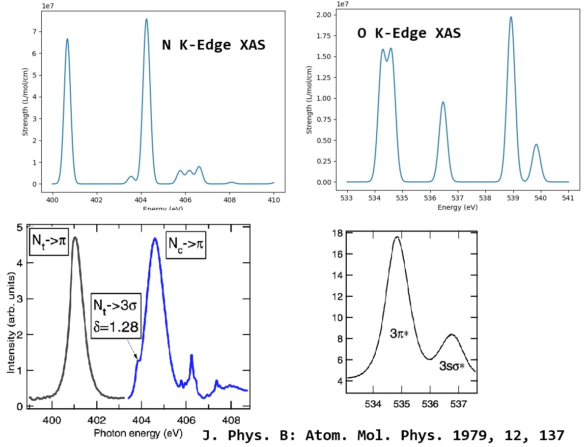
We can see that, MSDFT can give quite good results for N and O K-edge XAS!