All input and output files can be downloaded here.
Quantum Mechanics/Molecular Mechanics (QM/MM) Energy
This tutorial will lead you step by step to do QM/MM calculations using Qbics. Before proceeding, it is strongly recommended that you read the following 2 tutorials first:
For a QM/MM calculation, you should first prepare the topology and parameters for the whole system like in MM calculations, then assign the QM region, set QM options, then a calculation can be done.
Abscisic Acid in Water Sphere
The abscisic acid (ABA) has been considered in Molecular Mechanics Energy. Now we want to study its microsolvation behaviour, and do a QM/MM calculation.
Solvating ABA into a Water Sphere
There are many ways of solvating a molecule into water or any other solvent. Here we use VMD.
- Copy
aba/aba.rtf,toppar/top_all36_cgenff.rtf, andligandrm.pdb,ligandrm.psfgenerated from Molecular Mechanics Energy to the current path (Assume it isc:\work(Windows) or/home/you/work(Linux)). - Before proceeding, an additional work needs to be done. If you open
ligandrm.pdb, you will find that the element line is blank. For MM calculations, this is not important. But for QM/MM calculations, this is highly dangerous since Qbics may fail to recognize what elements those atoms are. We must add correct elements in the 78th column, like this:
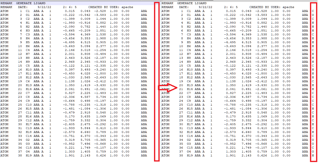
In Qbics, mol ... end can accept either explicit atom coordinates, XYZ files, or PDB files. In PDB files, the last column should be elements, but some programs generate PDB files with the last column left blank. For pure MM calculations, this does not matter. But for QM and QM/MM calculations, you MUST write element names there, otherwise the program may fail to identify the element.
- Open VMD, click
Extentions --> Tk Consoleto open the TkConsole. - Use the following command to switch to the current path:
$ cd c:/work        # Windows
$ cd /home/you/work # Linux- Prepare a TCL script called
wat_sphere.tclin the current path with the following content:
proc wat_sphere {molname max} {
    mol new ${molname}.psf
    mol addfile ${molname}.pdb
    set cen [measure center [atomselect top all] weight mass]
    set x1 [lindex $cen 0]
    set y1 [lindex $cen 1]
    set z1 [lindex $cen 2]
    mol delete top
    package require solvate
    solvate ${molname}.psf ${molname}.pdb -t [expr $max+5] -o del_water
    resetpsf
    package require psfgen
    mol new del_water.psf
    mol addfile del_water.pdb
    readpsf del_water.psf
    coordpdb del_water.pdb
    set wat [atomselect top "same residue as {water and ((x-$x1)*(x-$x1) + (y-$y1)*(y-$y1) + (z-$z1)*(z-$z1))<($max*$max)}"]
    set del [atomselect top "water and not same residue as {water and ((x-$x1)*(x-$x1) + (y-$y1)*(y-$y1) + (z-$z1)*(z-$z1))<($max*$max)}"]
    set seg [$del get segid]
    set res [$del get resid]
    set name [$del get name]
    for {set i 0} {$i < [llength $seg]} {incr i} {
      delatom [lindex $seg $i] [lindex $res $i] [lindex $name $i]
    }
    writepsf ${molname}_ws.psf
    writepdb ${molname}_ws.pdb
    mol delete top
 }
This script use both TCL grammar and some VMD extensions. It can be used to solvate any molecules into a water sphere.
- Now in the TkConsolve, type the following commands:
$ source wat_sphere.tcl
$ wat_sphere ligandrm 20
The function wat_sphere will use ligandrm.pdb and ligandrm.psf to build a system of ABA solvating into a water sphere of radius 20 Angstrom. After a few seconds, you will get ligandrm_ws.pdb and ligandrm_ws.psf. Open ligandrm_ws.pdb, you will see that ABA has indeed be solvated:
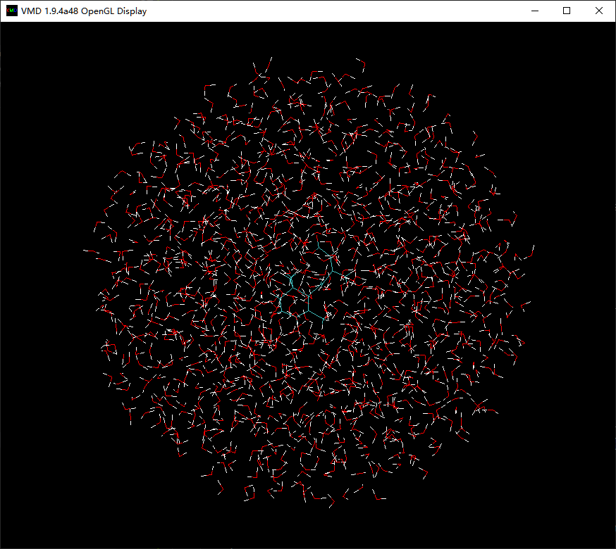
As done above, in the 78th column of ligandrm_ws.pdb, you must add correct elements.
Calculating Energy: ABA
Now we can do a QM/MM calculation. The QM region is just ABA.
- Copy
ligandrm_ws.pdb,ligandrm_ws.psf,par_all36_cgenff.prm,aba.prm, andtoppar_water_ions.str(see Molecular Mechanics Energy) in to the current path. We needtoppar_water_ions.strbecause it contains paramters for water, which is absent inpar_all36_cgenff.prm. - So we can provide the following input:
charmm
    parameters par_all36_cgenff.prm aba.prm toppar_water_ions.str
    topology   ligandrm_ws.psf
    scaling14  1
    rcutoff    15.0
    rswitch    16.0
end

basis
    def2-svp
end

scf
    charge  -1 # ABA is negatively charged.
    spin2p1 1
    type    R
end

grimmedisp
    type bj
end

mol
    ligandrm_ws.pdb
end

qmmm
    qm_region  1-38
end

task
    energy b3lyp/charmm
end
You can see that, we just write QM and MM options to set up our calculation. There are a few tips:
- For gas phase QM/MM calculations,
rswitchmust be greater thanrcutoffsince it is unnecessary to use cut off distance. - You need to assign QM region by giving its atom indices in
qmmm ... endblock,qm_regionoption. - Remember that ABA is negatively charged, so
chargeshould be-1.
This is a B3LYP-D3BJ/SVP/CHARMM calculation for ABA in water sphere. There are 3506 atoms, 38 of which are treated quatnum mechanically. Run the calculation:
$ qbics aba_qmmm.inp -n 4 > aba_qmmm.out In the output file, you can see both QM- and MM-related quantities:
SCF Energies
============
Kinetic energy:                             874.28910347 Hartree
Electron-nuclear attraction energy:       -5069.16661599 Hartree
Pseudopotential energy:                       0.00000000 Hartree
Exchange-correlation energy:                -99.51029771 Hartree
Electron Coulomb energy:                   1936.49539372 Hartree
Electron exchange energy:                   -23.48991459 Hartree
Nuclear repulsion energy:                  1495.38867451 Hartree
Grimme dispersion energy:                    -0.08299289 Hartree
----------------------------------------------------------------
SCF energy (E):                            -886.07664949 Hartree
Virial quotien (V/T):                        -2.01348244

Molecular Orbitals
==================
...
CHARMM energies
===============
Bond energy:                 1078.71984902 kcal/mol
Angle energy:                 259.35234584 kcal/mol
Dihedral energy:               35.62171511 kcal/mol
Improper energy:                0.08140330 kcal/mol
Coulombic energy:          -11343.24793116 kcal/mol
Lennard-Jones energy:        1004.38787762 kcal/mol
---------------------------------------------------
CHARMM energy:              -8965.08474028 kcal/mol

Total QM/MM energy
==================
Polarized QM energy:       -886.07664949 Hartree
Whole system MM energy:     -14.28677204 Hartree
QM/MM energy correction:      2.60722562 Hartree
------------------------------------------------
QM/MM energy:              -897.75619591 Hartree

Final total energy:        -897.75619591 Hartree
So, the total QM/MM energy is -897.75619591 Hartree.
Protein: With Boundary Bonds, Using PHO
In this section, we will do a QM/MM calculation for a protein, with a few residues in QM region.
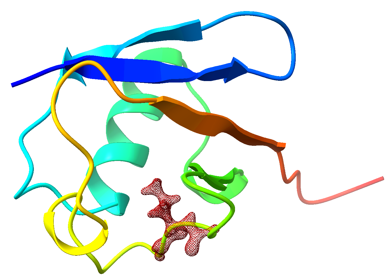
We will use ubiquitin in Molecular Mechanics Energy as an example. In the package downloaded from CHARMM-GUI, you can find step1_pdbreader.pdb and step1_pdbreader.psf, they the coordinates and topology of the protein.
Assume we want to treat Leu50 quantum mechanically and remaining atoms molecular mechanically, it seems that we can simply write the atom indices of Leu50 to qmmm ... end block. However, this is not a suitable way. Since there are covalent bonds between Leu50 and remaining parts, special treatments are needed. We need to use a method exclusive in Qbics, called projected hybrid orbitals (PHO) to treat such cases.
PHO is a powerful method, using complicated transformations to treat boundary covalent bonds. But at the same time, Qbics has wrapped this method a black-box, so you can use it as you are doing ordinary SCF calculations. The only constraint is: the boundary atoms must be sp3 carbon.
The atomic indices of Leu50 is 794-812, the backbone carbon atoms in neighboring residues are sp3 ones, so it is logical to cut covalent bonds there. Their atomic indices are shown below:
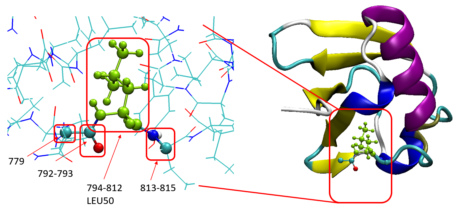
So, finally, the QM region is set to be 779 792-815. Now we can do the QM/MM calculations with PHO.
- In
step1_pdbreader.pdb, add element names at 78th column. See below.

- Prepare the input file:
charmm
    parameters par_all36m_prot.prm
    topology   step1_pdbreader.psf
    scaling14  1.0
    rcutoff    12.0
    rswitch    13.0
end

basis
    def2-svp
end

scf
    charge  0
    spin2p1 1
    type    R
end

grimmedisp
    type bj
end

qmmm
    qm_region  779 792-815
end

mol
    step1_pdbreader.pdb
end

task
    energy b3lyp/charmm
end
This will treat atoms 779 792-815 quantum mechanically and remaining atoms molecular mechanically. The boundary covalent bonds can be treated in a reasonable way by PHO method, and you do not need to do anything additionally!
Now run the calculation:
$ qbics protein-qmmm.inp -n 4 > protein-qmmm.outThe energis in protein-qmmm.out are shown below:
SCF Energies
============
Kinetic energy:                             605.07595152 Hartree
Electron-nuclear attraction energy:       -2971.45070239 Hartree
Pseudopotential energy:                       0.00000000 Hartree
Exchange-correlation energy:                -67.96939268 Hartree
Electron Coulomb energy:                   1064.79857616 Hartree
Electron exchange energy:                   -15.88462877 Hartree
Nuclear repulsion energy:                   774.61095516 Hartree
Grimme dispersion energy:                    -0.04599306 Hartree
----------------------------------------------------------------
SCF energy (E):                            -610.86523404 Hartree
Virial quotien (V/T):                        -2.00956786
...
CHARMM energies
===============
Bond energy:                  192.17336219 kcal/mol
Angle energy:                 296.89983569 kcal/mol
Dihedral energy:              730.62702525 kcal/mol
Improper energy:               10.75665901 kcal/mol
Coulombic energy:           -1832.30710714 kcal/mol
Lennard-Jones energy:         326.10889625 kcal/mol
---------------------------------------------------
CHARMM energy:               -275.74132875 kcal/mol

Total QM/MM energy
==================
Polarized QM energy:       -610.86523404 Hartree
Whole system MM energy:      -0.43942178 Hartree
QM/MM energy correction:      3.36386115 Hartree
------------------------------------------------
QM/MM energy:              -607.94079467 Hartree

Final total energy:        -607.94079467 Hartree
We now try to visualize the QM/MM wavefunction, for example, electron density. Open protein-qmmm.mwfn with Multiwfn and type:
$ Multiwfn protein-qmmm.mwfn
$ 5
$ 1
$ 2
$ 2
Then you will get a Gaussian cube file density.cub, which is the electron density obtained from the above QM/MM calculations. Note that in protein-qmmm.mwfn there are only atoms in QM region. If you open density.cub and step1_pdbreader.pdb together in a program, like Chimera or VMD, you can see that the electron density is indeed in the protein:
