Tip
All input files can be downloaded: Files.
Tip
For more information of this section, please refer to these pages:
Prediction of the Inverted Singlet-Triplet (IST) Energy Gap Using TSO-DFT
Hund’s rule argues that for the same electron configuration, the term with the highest spin multiplicity is more stable. In the case of electrofluorescence, this means that the triplet state is more stable than the singlet state. Define the gap:
\(\Delta E = E_{S_1} - E_{T_1}\)
Then, in moste cases, \(\Delta E > 0\). However, violations of Hund’s rule have been experimentally observed for a special class of materials, i.e., they have negative \(\Delta E\) or inverted singlet-triplet (IST) energy gap. They are very important for triplet harvesting via reverse intersystem crossing (RISC).
In J. Phys. Chem. Lett. 2026, 17, 6233, the paper uses TSO-DFT to calculate excitation energies of molecules containing IST signatures with the B3LYP functional. For more than 34 molecules, TSO-DFT gives relialbe negative \(\Delta E < 0\). The paper argues that “The TSO-DFT methodology (with the B3LYP functional), benchmarked against experimentally reported and theoretically proposed IST molecules, shows superior accuracy in predicting negative ΔEST compared to standard EOM-CCSD and ADC(2) methods, establishing it as a uniquely cost-effective tool for IST emitter design.”
In this tutorial, we will use Qbics to reproduce one \(\Delta E\) of this paper.
Molecular Structure Optimization
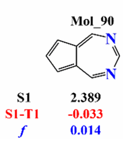
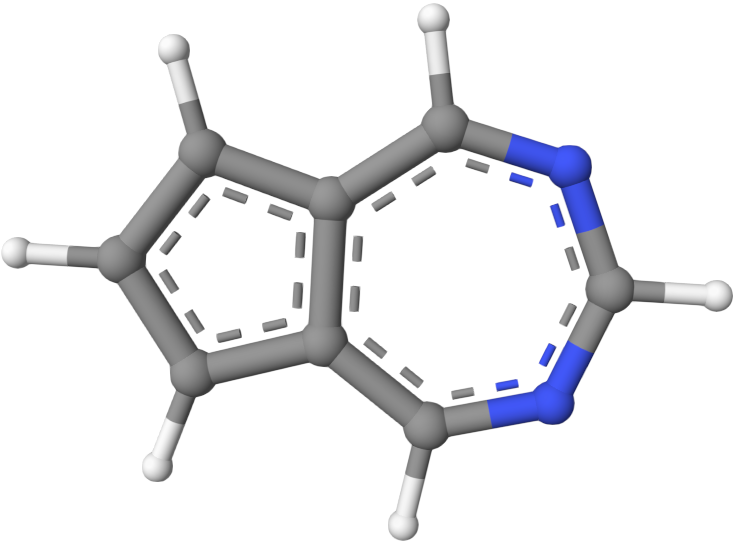
We want to reprocude this molecule:
First we want to optimize the geometry of the molecule. Although there are a lot of ways, the best way is to use Qbics-MolStar. Follow the way below:
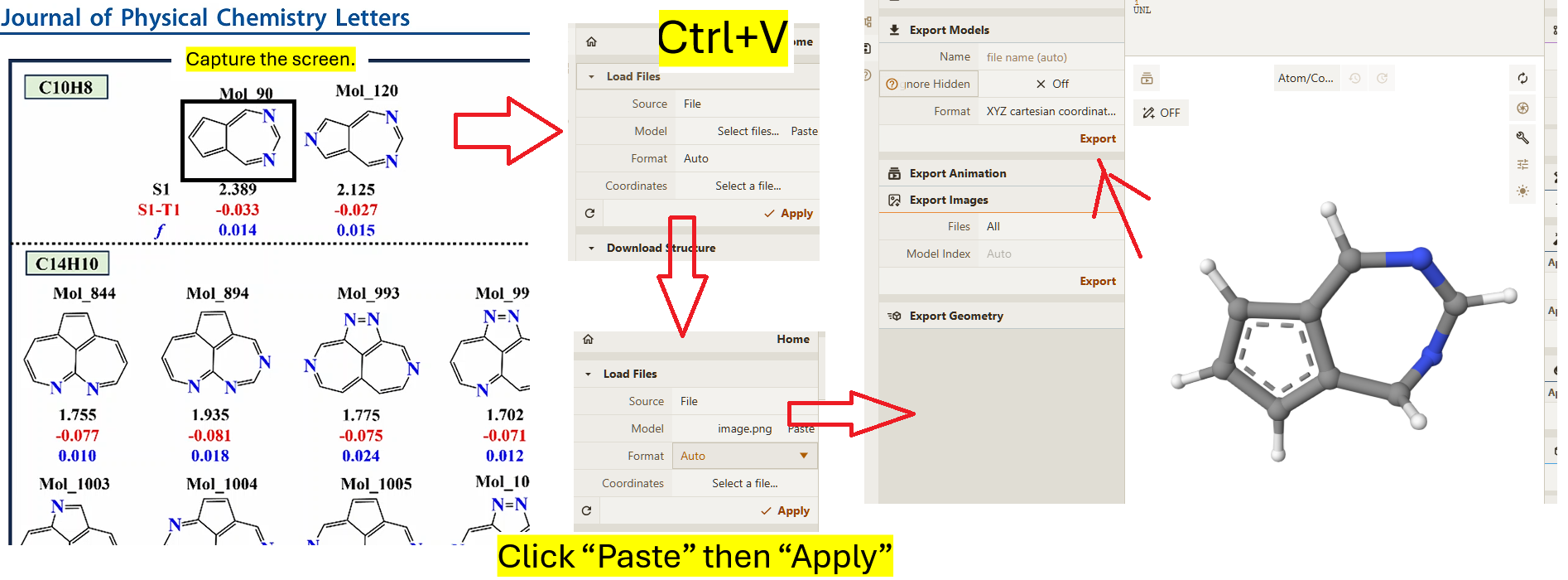
The AI system MolScribe can transform the graph into SMILES then 3D coordinates. Export it to an XYZ file, then we can optimize it with DFT:
 1mol
 2C           -1.04156270504793        0.06898020823976        0.09869238425253
 3C           -0.72238817674403       -1.15931457328814        0.67284176885867
 4C            0.63394793033020       -1.41302316734170        0.46159998923951
 5C            1.41478346893870       -2.42805267506438        1.00117167387101
 6N            2.62245417676414       -2.79584357351428        0.63367340475859
 7C            3.41685931263871       -2.16430942452300       -0.20237887757826
 8N            3.49473417039696       -0.89689038258302       -0.54452997202527
 9C            2.52445541954071       -0.00971319464880       -0.49597854021721
10C            1.17406324852518       -0.23762406158590       -0.26383605635284
11C            0.10653975781569        0.64549780746266       -0.43849152071242
12H           -2.01697624661691        0.52188693363575        0.10703595430576
13H           -1.40230168786037       -1.81247909433718        1.18746051037906
14H            0.97337005914902       -3.06388117737919        1.76387738499715
15H            4.22918260936383       -2.77655184028781       -0.58722807896853
16H            2.83678247125013        0.99905528682127       -0.75177723589980
17H            0.16805619155599        1.60526292839398       -0.91713278890795
18end
19
20scf
21    charge  0
22    spin2p1 1
23end
24
25basis
26    def2-svp
27end
28
29task
30    opt b3lyp
31end
Run the calculation:
$ qbics mol.inp -n 8 > mol.out
Here, -n 8 means Qbics will use 8 CPU cores for parallization. You can use any number of CPU cores you want. This file:
mol-opt.xyz: The optimized structure.
It can be used for the following calculations. You can view mol-opt.xyz with Qbics-MolStar:
Ground State (\(S_0\))
For the ground state of the moledcule, the input file is:
 1mol
 2    C     -1.05021810      0.11005247      0.20901148
 3    C     -0.72792887     -1.15307286      0.74230658
 4    C      0.63363616     -1.40430001      0.48611827
 5    C      1.36824481     -2.53547328      0.84094269
 6    N      2.64920463     -2.83059178      0.62089769
 7    C      3.54719215     -2.07221189     -0.01173141
 8    N      3.52290245     -0.87107265     -0.59413879
 9    C      2.47246947     -0.05579931     -0.69203622
10    C      1.16140992     -0.22045975     -0.24340688
11    C      0.09104098      0.68119251     -0.38705483
12    H     -2.03498639      0.57802698      0.25387230
13    H     -1.40786402     -1.82681691      1.26360528
14    H      0.81471500     -3.31384208      1.38766742
15    H      4.54007164     -2.54570028     -0.06114850
16    H      2.68670958      0.89074036     -1.21044980
17    H      0.14540060      1.65232848     -0.87945526
18end
19
20scf
21    charge  0
22    spin2p1 1
23end
24
25basis
26    def2-svp
27end
28
29task
30    energy b3lyp
31end
This is a standard file for DFT calculation of the singlet ground state of the molecule. See Density Functional Theory Calculations for more information. Run the calculation:
$ qbics s0.inp -n 8 > s0.out
Here, -n 8 means Qbics will use 8 CPU cores for parallization. You can use any number of CPU cores you want. There will be 2 output files:
s0.out: The output file of the DFT calculation.s0.mwfn: The wave function file.
In s1.out, you will find the energy:
1Final total energy: -417.60299721 Hartree
Triplet State (\(T_1\))
In the same way, we can calculate the triplet ground state of the molecule. The input file is:
 1mol
 2    C     -1.05021810      0.11005247      0.20901148
 3    C     -0.72792887     -1.15307286      0.74230658
 4    C      0.63363616     -1.40430001      0.48611827
 5    C      1.36824481     -2.53547328      0.84094269
 6    N      2.64920463     -2.83059178      0.62089769
 7    C      3.54719215     -2.07221189     -0.01173141
 8    N      3.52290245     -0.87107265     -0.59413879
 9    C      2.47246947     -0.05579931     -0.69203622
10    C      1.16140992     -0.22045975     -0.24340688
11    C      0.09104098      0.68119251     -0.38705483
12    H     -2.03498639      0.57802698      0.25387230
13    H     -1.40786402     -1.82681691      1.26360528
14    H      0.81471500     -3.31384208      1.38766742
15    H      4.54007164     -2.54570028     -0.06114850
16    H      2.68670958      0.89074036     -1.21044980
17    H      0.14540060      1.65232848     -0.87945526
18end
19
20scf
21    charge  0
22    spin2p1 3
23end
24
25basis
26    def2-svp
27end
28
29task
30    energy b3lyp
31end
Run the calculation:
$ qbics t1.inp -n 8 > t1.out
In t1.out, you will find the energy:
1Final total energy: -417.49957900 Hartree
Usually, the triplet state can be calculated in this way. However, in the case of IST molecules, it is known that the calculation of triplet state can lead often lead to high-energy solutions. Therefore, it is recommended that the triplet state calculation should use the ground state wave function as initial guess. Thus, we use s0.mwfn obtained in the last calculation as initial guess (see scfguess for more information). The input file is:
 1mol
 2    C     -1.05021810      0.11005247      0.20901148
 3    C     -0.72792887     -1.15307286      0.74230658
 4    C      0.63363616     -1.40430001      0.48611827
 5    C      1.36824481     -2.53547328      0.84094269
 6    N      2.64920463     -2.83059178      0.62089769
 7    C      3.54719215     -2.07221189     -0.01173141
 8    N      3.52290245     -0.87107265     -0.59413879
 9    C      2.47246947     -0.05579931     -0.69203622
10    C      1.16140992     -0.22045975     -0.24340688
11    C      0.09104098      0.68119251     -0.38705483
12    H     -2.03498639      0.57802698      0.25387230
13    H     -1.40786402     -1.82681691      1.26360528
14    H      0.81471500     -3.31384208      1.38766742
15    H      4.54007164     -2.54570028     -0.06114850
16    H      2.68670958      0.89074036     -1.21044980
17    H      0.14540060      1.65232848     -0.87945526
18end
19
20scf
21    charge  0
22    spin2p1 3
23end
24
25scfguess
26    type mwfn
27    file s0.mwfn
28end
29
30basis
31    def2-svp
32end
33
34task
35    energy b3lyp
36end
Run the calculation:
$ qbics t1-s0guess.inp -n 8 > t1-s0guess.out
In t1-s0guess.out, you will find the energy:
1Final total energy: -417.51425840 Hartree
This energy is lower than the one shown in t1.out`, which is what we need.
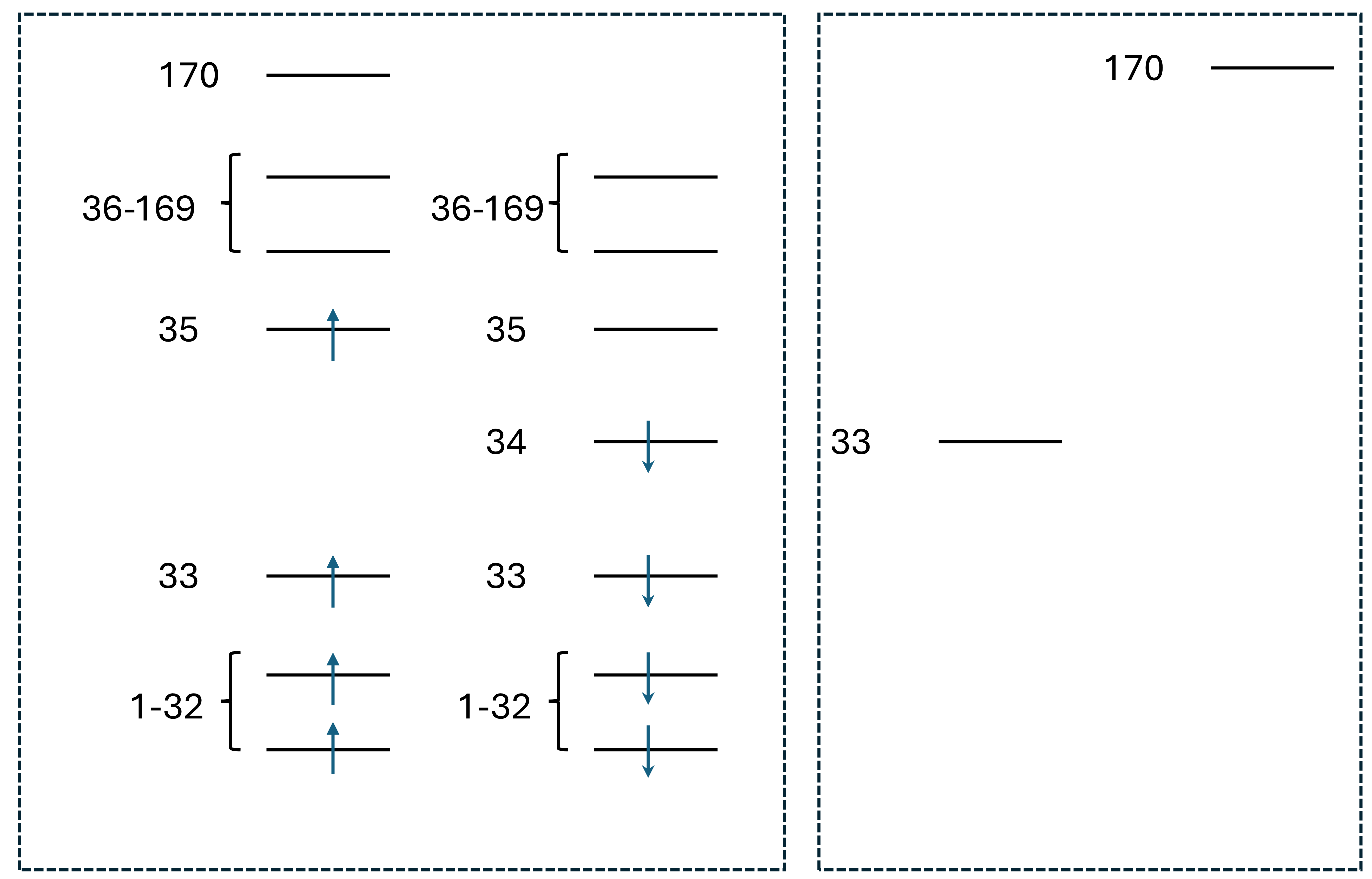
We can also check the orbital occupation in t1-s0guess.out:
132         1.000          -0.28040102         1.000          -0.25316116
233         1.000          -0.27169404         1.000          -0.24475506
334         1.000          -0.24605069         0.000          -0.18938584
435         1.000          -0.14796951         0.000          -0.07173325
536         0.000          -0.09171801         0.000          -0.06178308
637         0.000           0.01880794         0.000           0.05227252
738         0.000           0.05986264         0.000           0.06209003
So, there are 2 singly occupied orbitals: 34 and 35.
Singlet Excited State (\(S_1\))
Now we will calculate \(S_1\), where the 2 singly occupied orbitals are still 34 and 35, but they coupled to a singlet state. The input file is
 1mol
 2    C     -1.05021810      0.11005247      0.20901148
 3    C     -0.72792887     -1.15307286      0.74230658
 4    C      0.63363616     -1.40430001      0.48611827
 5    C      1.36824481     -2.53547328      0.84094269
 6    N      2.64920463     -2.83059178      0.62089769
 7    C      3.54719215     -2.07221189     -0.01173141
 8    N      3.52290245     -0.87107265     -0.59413879
 9    C      2.47246947     -0.05579931     -0.69203622
10    C      1.16140992     -0.22045975     -0.24340688
11    C      0.09104098      0.68119251     -0.38705483
12    H     -2.03498639      0.57802698      0.25387230
13    H     -1.40786402     -1.82681691      1.26360528
14    H      0.81471500     -3.31384208      1.38766742
15    H      4.54007164     -2.54570028     -0.06114850
16    H      2.68670958      0.89074036     -1.21044980
17    H      0.14540060      1.65232848     -0.87945526
18end
19
20scf
21    charge  0
22    spin2p1 1
23    type    U
24    no_scf  tso
25end
26
27scfguess
28    type mwfn
29    file s0.mwfn
30    orb 68 1 1-33 35-170 : 1-169
31    orb  0 1          34 : 170
32end
33
34basis
35    def2-svp
36end
37
38task
39    energy b3lyp
40end
For more details about TSO-DFT, please refer to TSO-DFT (1): Excited States and scfguess. Here we give a brief introduction:
Line 24: We set
no_scftotsoto use TSO-DFT.Line 23: TSO-DFT must use unrestricted SCF, so we set
typetoU.Line 28-29: We use the \(S_0\) state as the initial guess.
Line 30-31: The orbital opartition for calculating \(S_1\) state. For more details, see TSO-DFT (1): Excited States. Briefly, orbitals are partitioned into 2 subspaces as shown below, one is the orbitals removing alpha 34 and beta 170 (the highest one, to ensure the number of alpha and beta orbitals are the same), and this subspace has 68 electrons with the expected spin multiplicity 1. The other subspace is alpha 34 and beta 170, which has 0 electrons. Using this partition, the Aufbau occupation leads to a 34
Line 30-31: The orbital opartition for calculating \(S_1\) state. For more details, see TSO-DFT (1): Excited States. Briefly, orbitals are partitioned into 2 subspaces as shown below, one is the orbitals removing alpha 34 and beta 170 (the highest one, to ensure the number of alpha and beta orbitals are the same), and this subspace has 68 electrons with the expected spin multiplicity 1. The other subspace is alpha 34 and beta 170, which has 0 electrons. Using this partition, the Aufbau occupation leads to a 34 → 35 singlet excited state.
Run the calculation:
$ qbics s1.inp -n 8 > s1.out
In s1.out, you will find the output:
 1TSO Transition
 2==============
 3Reference wave function read from: s0.mwfn
 4Reference energy:         -417.60299700 Hartree
 5Current energy:           -417.51546285 Hartree
 6E(Current)-E(Ref):           2.38192545 eV
 7Transition dipole moment (Debye):  -0.44664  -0.97920   0.60661
 8Oscillator strength:                0.01379
 9Higher order corrections:
10Transition quadrupole moment (Debye*Angstrom):
11 Qxx:  -1.42726; Qyy:   2.24129; Qzz:   0.10584
12 Qxy:  -1.06345; Qxz:   0.93535; Qyz:  -0.77974
13Quadrupole correction to oscillator strength: 8.60036E-09
14Transition angular momentum (au):   0.00000   0.00000   0.00000
15Magnetic dipole correction to oscillator strength: 0.00000E+00
16
17 ---- Self Consistent Field Energy Done ------------------
18
19Final total energy:        -417.51546285 Hartree
Here:
Line 5, 19: The final total energy of the \(S_1\) state is
-417.51546285Hartree.Line 6: The excitation energy relative to the ground state.
Line 8: The oscillator strength.
The Singlet-Triplet Gap
Now we can calculate the \(\Delta E\) of the molecule:
\(\Delta E = E_{S_1} - E_{T_1} = (-417.51546285 - (-417.51425840))*27.21 = -0.033\) eV
and the oscillator strength of \(S_1\) state is 0.01379. Both the gap and the strength are reproduced successfully!