Tip
All input files can be downloaded: Files.
Tip
For more information of this section, please refer to these keywords:
Multi-State Energy Decomposition Analysis for Exciplexes
This tutorial will lead you step by step to do multi-state energy decomposition analysis (MS-EDA) for exciplexes using Qbics.
Hint
If you use Qbics to do MS-EDA in you paper, please cite the following references:
Theory: How to Decompose the Exciplex Energy
Input
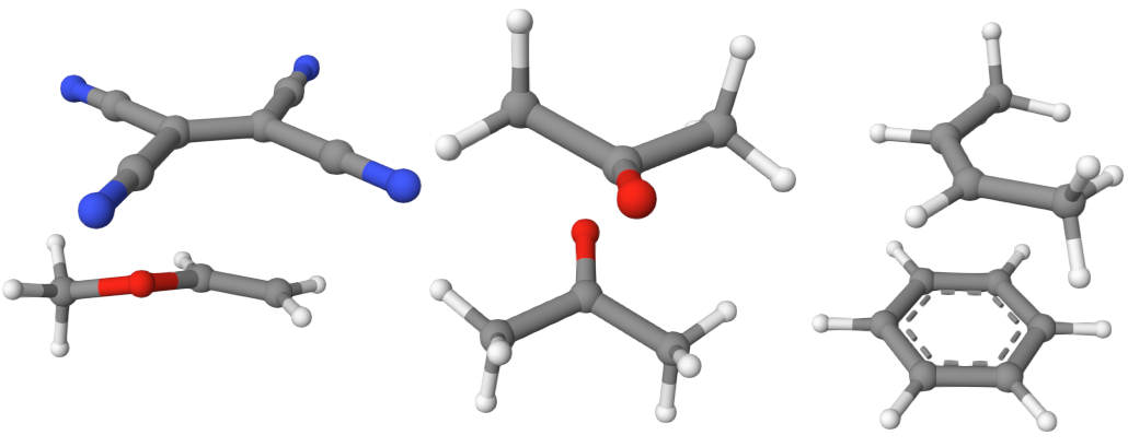
Below, we consider 3 exciplexes: (MeOCH=CH2)(TCNE), acetone dimer, and (C6H6)-(cis-2-butadiene).
Their input files are shown below:
 1mol
 2C      -0.198382       0.676975        0.839378
 3C      -1.315863       0.038931        0.405996
 4C      -2.225365       0.670286        -0.508436
 5N      -2.959552       1.174482        -1.247154
 6C      -1.634267       -1.289698       0.850726
 7N      -1.901673       -2.352749       1.221105
 8C      0.723624        0.024005        1.725081
 9N      1.483401        -0.507944       2.417545
10C      0.131547        2.005023        0.406927
11N      0.406859        3.079229        0.077027
12C      -0.018608       -1.360064       -2.097094
13C      1.086004        -1.277514       -1.352322
14H      -0.458263       -2.333443       -2.305731
15H      -0.471114       -0.462748       -2.522620
16H      1.590935        -2.157076       -0.934177
17O      1.621801        -0.078506       -1.011442
18C      2.981195        -0.123945       -0.597217
19H      3.629890        -0.409943       -1.438672
20H      3.239414        0.887438        -0.263120
21H      3.112168        -0.831294       0.237956
22end
23
24basis
25    cc-pvdz
26end
27
28scf
29    charge  0
30    spin2p1 1
31    type    u
32end
33
34eda
35    type mseda
36    frag 0 1  1-10
37    frag 0 1 11-20
38    # Orbital partition for fragment 1
39    orb1 64 1 1-31 33-140 : 1-139
40    orb1  0 1          32 : 140
41    orb1 32 1     141-226 : 141-226
42    # Orbital partition for fragment 2
43    orb2 64 1       1-140 : 1-140
44    orb2 32 1     141-155 157-226 : 141-225
45    orb2  0 1                 156 : 226
46    # Orbital partition for the whole molecule
47    orb 96 1 1-47 49-226 : 1-225
48    orb  0 1          48 : 226
49end
50
51task
52    eda m062x
53end
 1mol
 2 C                  1.40501800    0.00020500    0.16613500
 3 O                  1.96732200    0.00002100    1.32250100
 4 C                  1.50655000   -1.29318400   -0.61925100
 5 H                  2.50836500   -1.41216900   -1.04690200
 6 H                  1.29901100   -2.14677000    0.02291600
 7 H                  0.76955900   -1.24977400   -1.42041200
 8 C                  1.50473300    1.29462300   -0.61784400
 9 H                  2.50613100    1.41506600   -1.04604700
10 H                  0.76730100    1.25123500   -1.41860400
11 H                  1.29676400    2.14733100    0.02537900
12 C                 -1.57069600   -0.00057700   -0.15915200
13 O                 -1.45955200   -0.00147400   -1.36266600
14 C                 -1.67202400    1.28071400    0.63059600
15 H                 -0.94198800    1.27894000    1.44059400
16 H                 -1.51130700    2.13358300   -0.02305300
17 H                 -2.66412500    1.34977500    1.08181900
18 C                 -1.67029600   -1.28074500    0.63266100
19 H                 -1.50557100   -2.13424000   -0.01918900
20 H                 -0.94255800   -1.27573200    1.44471600
21 H                 -2.66346000   -1.35183900    1.08123100
22end
23
24basis
25    cc-pvdz
26end
27
28scf
29    charge  0
30    spin2p1 1
31    type    u
32end
33
34eda
35    type mseda
36    frag 0 1  1-10
37    frag 0 1 11-20
38    # Orbital partition for fragment 1
39    orb1  32 1 1-15 17-86 : 1-85
40    orb1   0 1         16 : 86
41    orb1  32 1     87-172 : 87-172
42    # Orbital partition for fragment 2
43    orb2  32 1           1-86 : 1-86
44    orb2  32 1 87-101 103-172 : 87-171
45    orb2   0 1            102 : 172
46    # Orbital partition for the whole molecule
47    orb  64 1 1-31 33-172 : 1-171
48    orb   0 1          32 : 172
49end
50
51task
52    eda m062x
53end
 1mol
 2C        -2.11437643657060   -0.85754420403449    0.63184430021191
 3C        -1.32991002940312   -1.39329844967993    1.63831931176558
 4C        -1.81293019105347    1.33073311710706    1.56276237609516
 5C        -2.35633843770169    0.50460524003657    0.59424676783581
 6H        -2.53847350527233   -1.50253884729794   -0.12405889027395
 7H        -1.14410843273496   -2.45741464148384    1.66881048558538
 8H        -2.00660926253103    2.39379539743948    1.53656866553163
 9H        -2.97003559294189    0.92298308733968   -0.19048089761824
10C        -1.02440574134394    0.79568848439314    2.56656836295313
11H        -0.59784058966710    1.44121012207980    3.32083332927968
12C        -0.78405589408731   -0.56662507682690    2.60499448062254
13H        -0.17129827655707   -0.98413854716428    3.39102605834755
14C         0.90530915148513    0.76859614859683   -0.69280985547464
15H         0.20967383636766    0.86860902650722   -1.51685088520083
16C         1.30597277062083   -0.44559901705687   -0.35097796744746
17H         0.92486814437303   -1.29036878583159   -0.91133975839400
18C         2.25957249832950   -0.81731353879967    0.73692864900559
19H         1.83711847972095   -1.62131069441208    1.33810967176003
20H         3.19277121604849   -1.18163197052739    0.30437410302004
21H         2.48581415297725    0.02130187194289    1.38838793614305
22C         1.30766703567951    2.06806699673986   -0.07669642598883
23H         1.87877136546791    2.65714541611658   -0.79526222872770
24H         0.41956249793524    2.63960219031429    0.18894978225370
25H         1.91208124086554    1.93108667450115    0.81435262871432
26end
27
28basis
29    cc-pvdz
30end
31
32scf
33    charge  0
34    spin2p1 1
35    type    u
36end
37
38eda
39    type mseda
40    frag 0 1  1-12
41    frag 0 1 13-24
42    # Orbital partition for fragment 1
43    orb1  42 1 1-20 22-114 : 1-113
44    orb1   0 1          21 : 114
45    orb1  32 1     115-210 : 115-210
46    # Orbital partition for fragment 2
47    orb2  42 1           1-114 : 1-114
48    orb2  32 1 115-129 131-210 : 115-209
49    orb2   0 1             130 : 210
50    # Orbital partition for the whole molecule
51    orb  74 1 1-36 38-210 : 1-209
52    orb   0 1          37 : 210
53end
54
55task
56    eda m062x
57end
We will take one example to explain the input, i.e., (MeOCH=CH2)(TCNE).
Before proceeding, you should have read TSO-DFT (1): Excited States to understand how to use TSO-DFT to get the excited states.
For the exciplex, we will use type mseda to do MS-EDA, and the fragments should be given by frag option. This is the same as the eda keyword in eda.
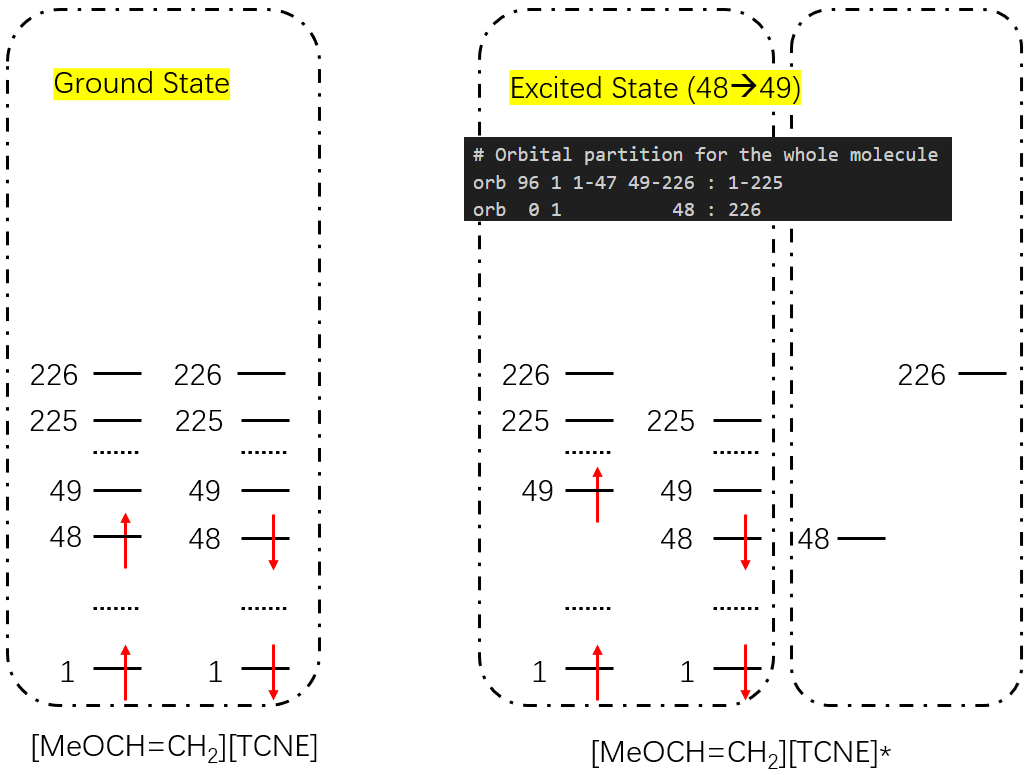
Now, we will use orb option to set the excited state of the whole exciplex. See Line 47-48. This is a 48 → 49 (HOMO → LUMO) singlet excited state. We partition the oribtals into 2 subspaces. By putting alpha 48 and beta 226 into a subspace with zero electrons, the Aufbau occupation of the first subspace naturally leads to the HOMO-LUMO transition. Of course, you can consider other excitations.
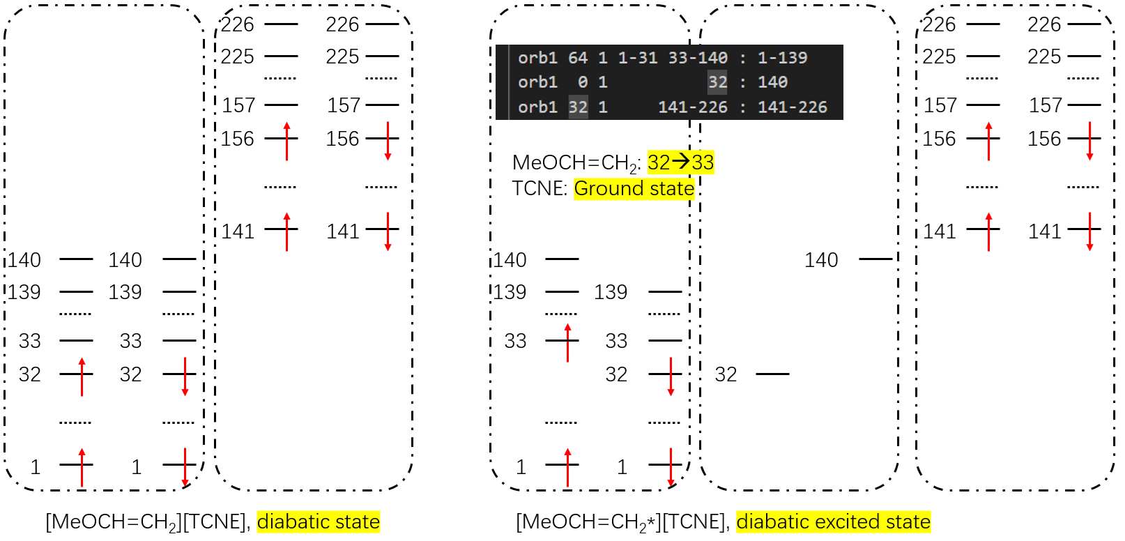
Then, we will use orb1 and orb2 options to set the diabatic excited states (MeOCH=CH2*)(TCNE) and (MeOCH=CH2)(TCNE*). See Line 39-41 and 43-45.
Below, in the left panel, we show the diabatic state of (MeOCH=CH2*)(TCNE), where the wave functions are localized on its own fragment. This state is assigned by frag automatically. In the right panel, we show the diabatic excited state of (MeOCH=CH2*)(TCNE). We partition the orbitals into 3 subspaces. By putting alpha 32 and beta 140 into a subspace with zero electrons, the Aufbau occupation of the first subspace naturally leads to the HOMO-LUMO transition of MeOCH=CH2. For the third subspace, we keep it unchanged as in the diabatic state, so TCNE is in the ground state.
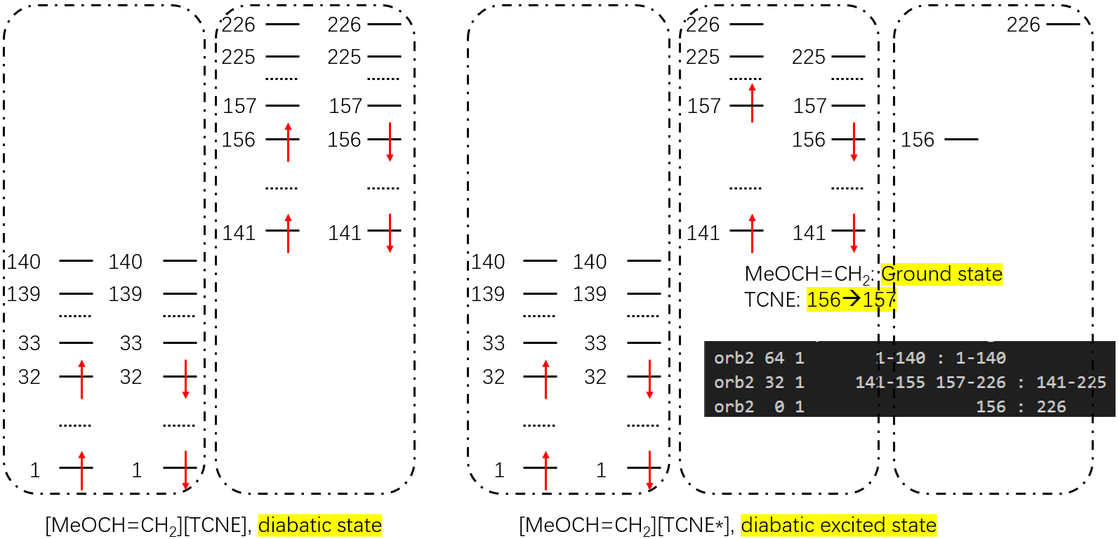
By the same logic, we can set the diabatic excited state of (MeOCH=CH2)(TCNE*) using orb2 option. See Line 43-45.
Finally, we can calculate the exciplex energy using eda m062x in the task section.
Here, we want to study the relationship between the HOMO-LUMO transition of the exciplex and the HOMO-LUM transition of the fragments. You can set orb1 and orb2 options to use other excited states.
For the other two exciplexes, the input files are written in the same way.
Output
After running the calculation, we will get the following output files. We again take (MeOCH=CH2)(TCNE) as an example.
 1---- NOSI Results ----
 2======================
 3   State   NOSI Energies  Excited Energy       Osc. Str.        DX        DY        DZ
 4               (Hartree)            (eV)                    (a.u.)    (a.u.)    (a.u.)
 5       0   -640.36742765      0.00000000      0.00000000  -0.96550   0.43709   0.00378
 6       1   -640.32444246      1.16962698      0.00000331  -0.01186  -0.00940  -0.00159
 7       2   -640.25510627      3.05626471      0.00000000   0.00000   0.00000   0.00000
 8       3   -640.15547535      5.76722204      0.00000000   0.00000   0.00000   0.00000
 9
10---- NOSI State Identification (Coefficients) ----
11==================================================
12State |0> = +0.707 |tn-Ax.B.mwfn> -0.707 |spin_flip_tn-Ax.B.mwfn>
13State |1> = -0.707 |tn-A.Bx.mwfn> +0.707 |spin_flip_tn-A.Bx.mwfn>
14State |2> = -0.698 |tn-Ax.B.mwfn> -0.698 |spin_flip_tn-Ax.B.mwfn> +0.111 |tn-A.Bx.mwfn> +0.111 |spin_flip_tn-A.Bx. mwfn>
15State |3> = +0.111 |tn-Ax.B.mwfn> +0.111 |spin_flip_tn-Ax.B.mwfn> +0.698 |tn-A.Bx.mwfn> +0.698 |spin_flip_tn-A.Bx. mwfn>
16--omitted--
17---- NOSI Results ----
18======================
19   State   NOSI Energies  Excited Energy       Osc. Str.        DX        DY        DZ
20               (Hartree)            (eV)                    (a.u.)    (a.u.)    (a.u.)
21       0   -640.36749379      0.00000000      0.00000000  -0.98365   0.43935   0.01448
22       1   -640.34091881      0.72310508      0.00000000   0.00000  -0.00000  -0.00000
23       2   -640.33660378      0.84051710      0.00145069   0.28743  -0.09118  -0.22446
24       3   -640.32372617      1.19091695      0.00009900   0.05373  -0.03170  -0.05398
25       4   -640.25509855      3.05827441      0.00000000   0.00000   0.00000   0.00000
26       5   -640.15527583      5.77445072      0.00000000   0.00000   0.00000   0.00000
27       6   -640.07534938      7.94924924      0.00077286  -0.02996   0.05389   0.06448
28       7   -640.07504770      7.95745814      0.00000000   0.00000  -0.00000  -0.00000
29
30---- NOSI State Identification (Coefficients) ----
31==================================================
32State |0> = -0.706 |tn-Ax.B.mwfn> +0.706 |spin_flip_tn-Ax.B.mwfn>
33State |1> = +0.705 |tn-A-.B+.mwfn> +0.705 |spin_flip_tn-A-.B+.mwfn>
34State |2> = -0.152 |tn-A.Bx.mwfn> +0.152 |spin_flip_tn-A.Bx.mwfn> -0.688 |tn-A-.B+.mwfn> +0.688 |spin_flip_tn-A-.B +.mwfn>
35State |3> = +0.691 |tn-A.Bx.mwfn> -0.691 |spin_flip_tn-A.Bx.mwfn> -0.168 |tn-A-.B+.mwfn> +0.168 |spin_flip_tn-A-.B +.mwfn>
36State |4> = +0.698 |tn-Ax.B.mwfn> +0.698 |spin_flip_tn-Ax.B.mwfn> -0.111 |tn-A.Bx.mwfn> -0.111 |spin_flip_tn-A.Bx. mwfn>
37State |5> = +0.111 |tn-Ax.B.mwfn> +0.111 |spin_flip_tn-Ax.B.mwfn> +0.699 |tn-A.Bx.mwfn> +0.699 |spin_flip_tn-A.Bx. mwfn>
38State |6> = +0.707 |tn-A+.B-.mwfn> -0.707 |spin_flip_tn-A+.B-.mwfn>
39State |7> = +0.707 |tn-A+.B-.mwfn> +0.707 |spin_flip_tn-A+.B-.mwfn>
40--omitted--
41---- NOSI Results ----
42======================
43   State   NOSI Energies  Excited Energy       Osc. Str.        DX        DY        DZ
44               (Hartree)            (eV)                    (a.u.)    (a.u.)    (a.u.)
45       0   -640.46151149      0.00000000      0.00000000  -1.39398   0.68556   0.39128
46       1   -640.34568876      3.15153658      0.00000000   0.00019   0.00008  -0.00003
47       2   -640.33525702      3.43538409      0.16461516  -1.15897   0.76059   1.41473
48
49---- NOSI State Identification (Coefficients) ----
50==================================================
51State |0> = -1.000 |tn-AB.mwfn>
52State |1> = -0.711 |tn-ABx.mwfn> +0.711 |spin_flip_tn-ABx.mwfn>
53State |2> = +0.703 |tn-ABx.mwfn> +0.703 |spin_flip_tn-ABx.mwfn>
54--omitted--
55MS-EDA Results
56==============
57E[A]+E[B] = -640.44244734 Hartree -> 0.00000 eV (as reference)
58E[A.B]    = -640.45105170 Hartree -> -0.23414 eV
59E[A+.B-]  = -640.07545516 Hartree -> 9.98637 eV
60E[A-.B+]  = -640.33851873 Hartree -> 2.82804 eV
61E[Ax.B]   = -640.31003238 Hartree -> 3.60319 eV
62E[A.Bx]   = -640.24118378 Hartree -> 5.47666 eV
63E[AB]     = -640.46138548 Hartree -> -0.51533 eV
64E[ABx]    = -640.34047390 Hartree -> 2.77484 eV
65
66      delta E_Lint =          E[A.B]-(E[A]+E[B]) = -0.00860437 Hartree = -0.23414 eV
67      delta E_exciton =       E[exciton]-E[A.B]
68delta delta E_superexchange = E[SE]-E[exciton]
69delta delta E_OCD =           E[es]-E[SE]
70
71For E[es], E[SE], and E[exciton], you will have to manually select from "NOSI Results" according to "NOSI State Identification (Coefficients)".
 1---- NOSI Results ----
 2======================
 3   State   NOSI Energies  Excited Energy       Osc. Str.        DX        DY        DZ
 4               (Hartree)            (eV)                    (a.u.)    (a.u.)    (a.u.)
 5       0   -386.02163213      0.00000000      0.00000000   0.39326  -0.00146  -0.23314
 6       1   -386.00338586      0.49648108      0.00000000  -0.00000   0.00000  -0.00000
 7       2   -385.97347538      1.31034511      0.00000035   0.00154   0.00000   0.00445
 8       3   -385.95321735      1.86156604      0.00000000  -0.00000  -0.00000  -0.00000
 9---- NOSI State Identification (Coefficients) ----
10==================================================
11State |0> = -0.707 |a2-Ax.B.mwfn> +0.707 |spin_flip_a2-Ax.B.mwfn>
12State |1> = +0.707 |a2-Ax.B.mwfn> +0.707 |spin_flip_a2-Ax.B.mwfn>
13State |2> = -0.707 |a2-A.Bx.mwfn> +0.707 |spin_flip_a2-A.Bx.mwfn>
14State |3> = -0.707 |a2-A.Bx.mwfn> -0.707 |spin_flip_a2-A.Bx.mwfn>
15--omitted--
16---- NOSI Results ----
17======================
18   State   NOSI Energies  Excited Energy       Osc. Str.        DX        DY        DZ
19               (Hartree)            (eV)                    (a.u.)    (a.u.)    (a.u.)
20       0   -386.02358380      0.00000000      0.00000000   0.27272  -0.00152  -0.23905
21       1   -386.00574867      0.48529396      0.00000000   0.00000  -0.00000   0.00000
22       2   -385.97730787      1.25916817      0.00001237   0.02577   0.00001   0.01185
23       3   -385.95818745      1.77943483      0.00000000  -0.00000  -0.00000  -0.00000
24       4   -385.86432757      4.33336215      0.00207198  -0.19771  -0.00008  -0.00760
25       5   -385.86302032      4.36893239      0.00000000   0.00000   0.00000   0.00000
26       6   -385.83882683      5.02723716      0.05642531   0.95823   0.00041   0.02725
27       7   -385.83832257      5.04095814      0.00000000  -0.00000  -0.00000  -0.00000
28
29---- NOSI State Identification (Coefficients) ----
30==================================================
31State |0> = -0.697 |a2-Ax.B.mwfn> +0.697 |spin_flip_a2-Ax.B.mwfn>
32State |1> = -0.695 |a2-Ax.B.mwfn> -0.695 |spin_flip_a2-Ax.B.mwfn> +0.083 |a2-A+.B-.mwfn> +0.083 |spin_flip_a2-A+.B-.mwfn>
33State |2> = -0.684 |a2-A.Bx.mwfn> +0.684 |spin_flip_a2-A.Bx.mwfn> +0.130 |a2-A-.B+.mwfn> -0.130 |spin_flip_a2-A-.B+.mwfn>
34State |3> = -0.674 |a2-A.Bx.mwfn> -0.674 |spin_flip_a2-A.Bx.mwfn> +0.162 |a2-A-.B+.mwfn> +0.162 |spin_flip_a2-A-.B+.mwfn>
35State |4> = -0.190 |a2-A.Bx.mwfn> +0.190 |spin_flip_a2-A.Bx.mwfn> -0.697 |a2-A-.B+.mwfn> +0.697 |spin_flip_a2-A-.B+.mwfn>
36State |5> = -0.220 |a2-A.Bx.mwfn> -0.220 |spin_flip_a2-A.Bx.mwfn> -0.690 |a2-A-.B+.mwfn> -0.690 |spin_flip_a2-A-.B+.mwfn>
37State |6> = +0.705 |a2-A+.B-.mwfn> -0.705 |spin_flip_a2-A+.B-.mwfn>
38State |7> = +0.139 |a2-Ax.B.mwfn> +0.139 |spin_flip_a2-Ax.B.mwfn> +0.704 |a2-A+.B-.mwfn> +0.704 |spin_flip_a2-A+.B-.mwfn>
39--omitted--
40---- NOSI Results ----
41======================
42   State   NOSI Energies  Excited Energy       Osc. Str.        DX        DY        DZ
43               (Hartree)            (eV)                    (a.u.)    (a.u.)    (a.u.)
44       0   -386.12737900      0.00000000      0.00000000   0.69404  -0.00130   0.01149
45       1   -386.02210988      2.86437281      0.00000000   0.00002  -0.00005   0.00002
46       2   -386.00487812      3.33324890      0.00160706  -0.00014   0.19868   0.00014
47
48---- NOSI State Identification (Coefficients) ----
49==================================================
50State |0> = -1.000 |a2-AB.mwfn>
51State |1> = +0.707 |a2-ABx.mwfn> -0.707 |spin_flip_a2-ABx.mwfn>
52State |2> = +0.707 |a2-ABx.mwfn> +0.707 |spin_flip_a2-ABx.mwfn>
53
54---- NOSI State Identification (Weights) ----
55=============================================
56State |0> = 1.000 |a2-AB.mwfn>
57State |1> = 0.500 |a2-ABx.mwfn> 0.500 |spin_flip_a2-ABx.mwfn>
58State |2> = 0.500 |a2-ABx.mwfn> 0.500 |spin_flip_a2-ABx.mwfn>
59--omitted--
60MS-EDA Results
61==============
62E[A]+E[B] = -386.11739232 Hartree -> 0.00000 eV (As reference)
63E[A.B]    = -386.12242778 Hartree -> -0.13702 eV
64E[A+.B-]  = -385.84489824 Hartree -> 7.41494 eV
65E[A-.B+]  = -385.87243970 Hartree -> 6.66550 eV
66E[Ax.B]   = -386.01250458 Hartree -> 2.85414 eV
67E[A.Bx]   = -385.96335089 Hartree -> 4.19168 eV
68E[AB]     = -386.12737901 Hartree -> -0.27175 eV
69E[ABx]    = -386.01349416 Hartree -> 2.82721 eV
70
71      delta E_Lint =          E[A.B]-(E[A]+E[B]) = -0.00503546 Hartree = -0.13702 eV
72      delta E_exciton =       E[exciton]-E[A.B]
73delta delta E_superexchange = E[SE]-E[exciton]
74delta delta E_OCD =           E[es]-E[SE]
 1---- NOSI Results ----
 2======================
 3   State   NOSI Energies  Excited Energy       Osc. Str.        DX        DY        DZ
 4               (Hartree)            (eV)                    (a.u.)    (a.u.)    (a.u.)
 5       0   -389.17311402      0.00000000      0.00000000 -49.44221  32.46889 175.72001
 6       1   -389.13014230      1.16926051      0.00000022  -0.00221   0.00104  -0.00311
 7       2   -389.04224936      3.56082738      0.00000000  -0.00000  -0.00000  -0.00000
 8       3   -388.98001080      5.25433883      0.00000000   0.00000  -0.00000  -0.00000
 9
10---- NOSI State Identification (Coefficients) ----
11==================================================
12State |0> = +0.707 |da-A.Bx.mwfn> -0.707 |spin_flip_da-A.Bx.mwfn>
13State |1> = -0.707 |da-Ax.B.mwfn> +0.707 |spin_flip_da-Ax.B.mwfn>
14State |2> = +0.703 |da-Ax.B.mwfn> +0.703 |spin_flip_da-Ax.B.mwfn>
15State |3> = -0.703 |da-A.Bx.mwfn> -0.703 |spin_flip_da-A.Bx.mwfn>
16--omitted--
17---- NOSI Results ----
18======================
19   State   NOSI Energies  Excited Energy       Osc. Str.        DX        DY        DZ
20               (Hartree)            (eV)                    (a.u.)    (a.u.)    (a.u.)
21       0   -389.17333875      0.00000000      0.00000000 -49.45653  32.46933 175.73035
22       1   -389.13050228      1.16558039      0.00001142   0.01954   0.00112  -0.02047
23       2   -389.04660899      3.44831695      0.00000000  -0.00000  -0.00000   0.00000
24       3   -389.03138698      3.86250786      0.00840862  -0.34847  -0.01060   0.23810
25       4   -389.02868531      3.93602011      0.00000000   0.00000   0.00000  -0.00000
26       5   -388.98027936      5.25314614      0.00000000  -0.00000  -0.00000   0.00000
27       6   -388.97047941      5.51980273      0.00000000   0.00000  -0.00000   0.00000
28       7   -388.96978161      5.53879003      0.00161774  -0.13448  -0.01237   0.07533
29
30---- NOSI State Identification (Coefficients) ----
31==================================================
32State |0> = +0.706 |da-A.Bx.mwfn> -0.706 |spin_flip_da-A.Bx.mwfn>
33State |1> = -0.705 |da-Ax.B.mwfn> +0.705 |spin_flip_da-Ax.B.mwfn>
34State |2> = +0.600 |da-Ax.B.mwfn> +0.600 |spin_flip_da-Ax.B.mwfn> +0.097 |da-A.Bx.mwfn> +0.097 |spin_flip_da-A.Bx.mwfn> +0.342 |da-A-.B+.mwfn> +0.342 |spin_flip_da-A-.B+.mwfn>
35State |3> = +0.706 |da-A-.B+.mwfn> -0.706 |spin_flip_da-A-.B+.mwfn>
36State |4> = +0.369 |da-Ax.B.mwfn> +0.369 |spin_flip_da-Ax.B.mwfn> -0.610 |da-A-.B+.mwfn> -0.610 |spin_flip_da-A-.B+.mwfn>
37State |5> = -0.635 |da-A.Bx.mwfn> -0.635 |spin_flip_da-A.Bx.mwfn> +0.282 |da-A+.B-.mwfn> +0.282 |spin_flip_da-A+.B-.mwfn>
38State |6> = -0.292 |da-A.Bx.mwfn> -0.292 |spin_flip_da-A.Bx.mwfn> -0.647 |da-A+.B-.mwfn> -0.647 |spin_flip_da-A+.B-.mwfn>
39State |7> = -0.708 |da-A+.B-.mwfn> +0.708 |spin_flip_da-A+.B-.mwfn>
40--omitted--
41---- NOSI Results ----
42======================
43   State   NOSI Energies  Excited Energy       Osc. Str.        DX        DY        DZ
44               (Hartree)            (eV)                    (a.u.)    (a.u.)    (a.u.)
45       0   -389.30494836      0.00000000      0.00000000 -49.31280  32.52416 175.77907
46       1   -389.14670530      4.30579375      0.00000000  -0.00000   0.00000   0.00000
47       2   -389.01536102      7.87967170      0.49201856  -0.66872   2.07558  -0.59758
48
49---- NOSI State Identification (Coefficients) ----
50==================================================
51State |0> = -1.000 |da-AB.mwfn>
52State |1> = -0.707 |da-ABx.mwfn> +0.707 |spin_flip_da-ABx.mwfn>
53State |2> = +0.707 |da-ABx.mwfn> +0.707 |spin_flip_da-ABx.mwfn>
54--omitted--
55MS-EDA Results
56==============
57E[A]+E[B] = -389.30025849 Hartree -> 0.00000 eV (as reference)
58E[A.B]    = -389.30313645 Hartree -> -0.07831 eV
59E[A+.B-]  = -388.97113637 Hartree -> 8.95587 eV
60E[A-.B+]  = -389.03260717 Hartree -> 7.28316 eV
61E[Ax.B]   = -389.08586649 Hartree -> 5.83390 eV
62E[A.Bx]   = -389.07689636 Hartree -> 6.07799 eV
63E[AB]     = -389.30494829 Hartree -> -0.12762 eV
64E[ABx]    = -389.08103350 Hartree -> 5.96542 eV
65
66      delta E_Lint =          E[A.B]-(E[A]+E[B]) = -0.00287796 Hartree = -0.07831 eV
67      delta E_exciton =       E[exciton]-E[A.B]
68delta delta E_superexchange = E[SE]-E[exciton]
69delta delta E_OCD =           E[es]-E[SE]
For tn.out, we list the results of TSO-DFT for the diabatic and dibatic excited states. The E[exciton], E[SE], and E[es] have to be selected from the NOSI energies, like shown in Line 5-8, 21-28, and 45-47. In most cases, you should choose the lowest singlet states, where the coefficients of the wave function and its spin-flip one have the same sign. The selected states are highlighted. For example, for exciton, we choose State 2 (Line 14), it is a combination of local exciton state [A*][B] and [A][B*], its energy is given in Line 7. For SE, we choose State 1 (Line 33), it is a state of [A-][B+] and has little contributions from other states. For es, we choose State 3 (Line 47), it is the target excited state.
Tip
In principle, you can choose other intermediate excited states to see the SE or exciton effects, but you should be absolutely sure what you intend to do.
Now we can do the calculations accoding to the equations given in Line 66-69.
delta E_Lint = E[A.B]-(E[A]+E[B]) = -0.23 eV
delta E_exciton = E[exciton]-E[A.B] = (-640.25510627–640.45105170)*27.21 = +5.33 eV
delta delta E_superexchange = E[SE]-E[exciton] = (-640.34091881–640.25510627)*27.21 = -2.33 eV
delta delta E_OCD = E[es]-E[SE] = (-640.33525702–640.34091881)*27.21 = +0.15 eV
For other exciplexes, the calculations are done in the same way. The results are shown below:
Type |
(MeOCH=CH2)(TCNE) |
acetone dimer |
(C6H6)-(cis-2-butadiene) |
|---|---|---|---|
\(\Delta E_{\text{Lint}}\) |
-0.23 eV |
-0.14 eV |
-0.08 eV |
\(\Delta E_{\text{exciton}}\) |
+5.33 eV |
+3.24 eV |
+7.10 eV |
\(\Delta \Delta E_{\text{superexchange}}\) |
-2.33 eV |
-0.06 eV |
-0.12 eV |
\(\Delta \Delta E_{\text{OCD}}\) |
+0.15 eV |
+0.02 eV |
+0.85 eV |
We can see that:
(MeOCH=CH2)(TCNE) has a very large \(\Delta\Delta E_{\text{superexchange}}\), so it is a charge transfer excipler;
Acetone dimer has very small \(\Delta\Delta E_{\text{superexchange}}\) and \(\Delta\Delta E_{\text{OCD}}\), so it is an encounter excipler;
(C6H6)-(cis-2-butadiene) has a large \(\Delta E_{\text{OCD}}\), so it is a intimate excipler. This is not unexpected, since a Dield-Alder reaction is about to occur between the two fragments upon photochemical ways, thus there should be considerable orbital overlap, leading to a large \(\Delta\Delta E_{\text{OCD}}\).
Besides the output file, you can also find some MWFN files corresponding to the diabatic (tn-A.B.mwfn), dibatic excited (tn-Ax.B.mwfn, tn-A.Bx.mwfn), charge-transfer (tn-A+.B-.mwfn, tn-A-.B+.mwfn), and standard ground (tn-AB.mwfn) and excited state (tn-ABx.mwfn).